Pei-jian Zhou (周佩剑), Fu-jun Wang (王福军), Zheng-jun Yang (杨正军), Jie-gang Mou (牟介刚)

1.College of Water Resources and Civil Engineering, China Agricultural University, Beijing 100083, China

2.College of Mechanical Engineering, Zhejiang University of Technology, Hangzhou 310014, China,

E-mail: peijianzhou@gmail.com

Investigation of rotating stall for a centrifugal pump impeller using various SGS models＊

Pei-jian Zhou (周佩剑)1,2, Fu-jun Wang (王福军)1, Zheng-jun Yang (杨正军)1, Jie-gang Mou (牟介刚)2

1.College of Water Resources and Civil Engineering, China Agricultural University, Beijing 100083, China

2.College of Mechanical Engineering, Zhejiang University of Technology, Hangzhou 310014, China,

E-mail: peijianzhou@gmail.com

The accurate modeling and prediction of the rotating stall in a centrifugal pump is a significant challenge. One of the modeling techniques that can improve the accuracy of the flow predictions is the large eddy simulation (LES). The quality of the LES predictions depends on the sub-grid-scale (SGS) model implemented in the LES. This paper assesses the influence of various SGS models that are suitable for predicting rotating stall in a low-specific speed centrifugal pump impeller. The SGS models considered in the present work include the Smagorinsky model (SM), the dynamic Smagorinsky model (DSM), the dynamic non-linear model (DNM), the dynamic mixed model (DMM) and the dynamic mixed non-linear model (DMNM). The results obtained from these models are compared with the PIV and LDV experimental data. The analysis of the results shows that the SGS models have significant influences on the flow field. Among the models, the DSM, the DMM and the DMNM can successfully predict the“two-channel” stall phenomenon, but not the SM and the DNM. According to the simulations, the DMNM gives the best prediction on the mean velocity flow field and also indicates improvements for the simulation of the turbulent flow. Moreover, the high turbulent kinetic energy predicted by the DMNM is in the best agreement with the experiment data.

Centrifugal impeller, rotating stall, large eddy simulation, sub-grid-scale (SGS) model

Introduction

The rotating stall is a key issue for the stable operation of centrifugal pumps[1,2]. This phenomenon often occurs under a part load condition and is usually accompanied with a large flow separation and strong anisotropy, which serves as a very severe test for the flow simulation by turbulence models based on the linear eddy viscosity concept. It is a challenging task to accurately predict the rotating stall within a pump.

The improvements in the computer power make it possible to implement advanced models such as the LES to study the performance of pumps. The application of the LES for pumps becomes a widely used technique in recent years. Byskov et al.[3]applied the LES and the RANS models to a centrifugal pump impeller containing two bladed channels. The results indicate that the LES results are in superior agreement with the measurements as compared to the RANS ones, particularly at the stall point. Feng et al.[4]implemented the hybrid RANS-LES approach to predict a “two-channel” stall phenomenon in the impeller, where the RNGand SSG models fail to provide such predictions. Lucius and Brenner[5,6]used another hybrid RANS-LES method called the scaleadaptive simulation to determine the rotating stall in a centrifugal pump, while Hasmatuchi[7]also applied the same methodology to investigate the stall flow in a pump-turbine. Tao et al.[8]considered a novel rotating correction on the RANS, to improve the accuracy under the designed condition. However, a large deviation can still be observed during the stall flow. In the study presented by Braun[9], numerical investigations of the rotating stall in a pump-turbine were performed. The results indicate that the SSTmodel fails toaccurately reproduce the phenomenon. Pacot et al.[10]investigated the rotating stall phenomena in a pumpturbine under a part load condition. The results demonstrate that unlike the RANS approach, the LES is a powerful tool to predict the stall flow.

According to the literature, the reliability of the LES relies on the performance of the employed SGS model. The early work presented by Kato et al.[11]shows that the stall point predicted by the SM for a mixed-flow pump is at a slightly lower flow-rate ratio, as compared to the measurements. Posa et al.[12]tested the SM and the filtered structured function (FSF) model for a mixed-flow pump, and it is shown that the FSF model performs better for the complex flow under the off-design condition. Yang et al.[13]evaluated SGS models including the SM, the DSM and the DMM for the LES in a shrouded six-bladed centrifugal pump impeller under the design condition. Among the models, the DMM showed improvement in predictions of both the surface shear stress and the velocity distributions. Furthermore, Yang and Wang[14]proposed a dynamic mixed nonlinear model (DMNM) which combines the advantages of the DMM and the DNM. Their study shows that the DMNM can capture the detailed vortex characteristics more accurately. The SGS models have great effects on the rotating stall in a pump. According to the knowledge of the authors, it is still not clear which SGS model can provide better predictions under similar circumstances. It is an urgent task to evaluate the performance of various SGS models.

The present study investigates the performance of five SGS models (SM, DSM, DNM, DMM and DMNM) in the internal flow prediction of a low specific speed centrifugal pump impeller under the stall condition. Various features studied include velocities, vortices and the turbulent kinetic energy, and the results predicted by the SGS models are compared with available experimental data obtained from the PIV and the LDV.

1. Description of SGS models

In the LES, the effects of large-scale eddies are considered while small-scale eddies are modeled according to a pattern. Compared to the original N-S governing equations, the LES involves an additional SGS stress tensor termwithin the governing equation. This term can be modeled with various SGS models such as SM, DSM, DNM, DMM and DMNM.

1.1Smagorinsky model (SM)

One of the earliest SGS model is proposed by Smagorinsky[15]for weather report. It is referred to as SM. The stress term of the SGS can be computed as

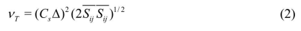
where the over-bar represents the spatial filter ring for a filtered sizeis the magnitude ofandis the Smagorinsky coefficient.

This model requires a small amount of computation and can be quite accurate in describing the subgrid dissipation characteristics. However, it has the following drawbacks:is a constant coefficient (the value of which depends on experience), it cannot describe the asymptotic behavior near the wall and it does not allow the SGS energy backscatter to the resolved scales.

1.2Dynamic Smagorinsky model (DSM)

Afterwards, a more comprehensive model (referred to as DSM) as compared to the SM was proposed[16]. This model overcomes some of the drawbacks of the SM and can be regarded as a modified SM[17]. The stress tensor can be expressed as

where the tilde denotes the test filtering at a test filter scaleis the resolved velocity componentis the SGS stress foris the so-called Leonard stress tensor which can be computed by the resolved scales.

Applying the SM to model the SGS stress, we have

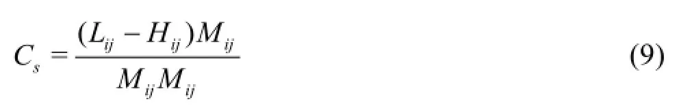
The DSM coefficient is calculated by using the least-squares method[15]

The DSM is one of the most popular SGS models due to its robustness, its ease to implement and the low computational cost. Also, it has many other desirable features, i.e., it requires only one input parameter,it has the correct asymptotic behavior near the wall and in laminar flows, and it does not prohibit the energy backscatter. However, the DSM has several aspects that require improvements. The model assumes that the SGS stress is only dependent on the resolved strain rate tensor. The principal axes of the SGS stress tensor are to be aligned with those of the resolved strain rate tensor. This model requires a slightly more computational time than the SM.

1.3Dynamic mixed model (DMM)

Singh and You[18]presented a DMM which employs a mixed model as the basis model. The anisotropic part of the SGS stress at a grid filter scale is expressed as follows

The anisotropic part of the SGS stress at a test filter scale is expressed as

The mixed SGS models have several advantages: (1) they require less sophisticated modeling due to the explicit calculation of the modified Leonard term, and only the residual stresses have to be modeled, (2) the modified Leonard term can provide the energy backscatter to the resolved scales, (3) the models will reduce the excessive backscatter represented by the eddy viscosity model which causes the previously mentioned numerical instability, and (4) they do not require alignment of the principal axes of the SGS stress tensor and the resolved strain rate tensor. Note that the DMM requires more computational time than the DSM.

1.4Dynamic non-linear model (DNM)

In the study presented by Yang et al.[19], the SGS was expressed in a general third-order formulation. In the current study, the modified cross term and the modified SGS Reynolds stress are modeled by using the following equation

The anisotropic part of the SGS stress at a test filter scale is expressed as:

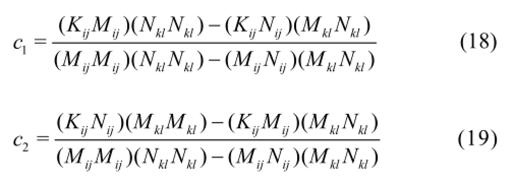
The two coefficients can be obtained by:

The SGS stress expression includes tensors of the resolved strain rate and the rotation rate, which represent the anisotropy of the rotating flows. Unlike the SM, it does not require an alignment between the SGS stress tensor and the resolved strain rate tensor. Also this model reflects both the forward and the backward scatters of the SGS turbulence kinetic energy between the filtered and the SGS motions, however, it does not consider the Leonard term. The amount of computations required by the DNM is almost the same as the DMM.

1.5Dynamic mixed non-linear model (DMNM)

Yang and Wang[14]developed a new model (known as DMNM) that retains the resolved modified Leonard term along with the modified expressions for the cross term and the SGS Reynolds stress. The SGS stress can be expressed as:

By substituting Eq.(15) and Eq.(16) into Eq.(3), the following equation is obtained

A similar approach in the DSM is implemented by using the least squares minimization of the error. The two coefficients in the DMNM are obtained by using the following equations:

This model combines the advantages of the DMM and the DNM, however, it needs the largest amount of computational time among the discussed SGS models. Yang and Wang[14]showed that the DMNM is more suitable for high curvature and strong rotational turbulence calculations as it considers the turbulent anisotropic properties.

2. The investigated pump impeller and simulation details

As shown in Fig.1, the considered pump impeller in this study is a shrouded, low specific-speed centrifugal impeller. The pump flow rate isand the head isunder the design condition. The simulation of the off-design condition(=Qis performed in this paper. The main geometry data of the impeller are summarized in Table 1. Note that more detailed geometry and experimental data are available in Ref.[20].

Fig.1 Geometry of the impeller

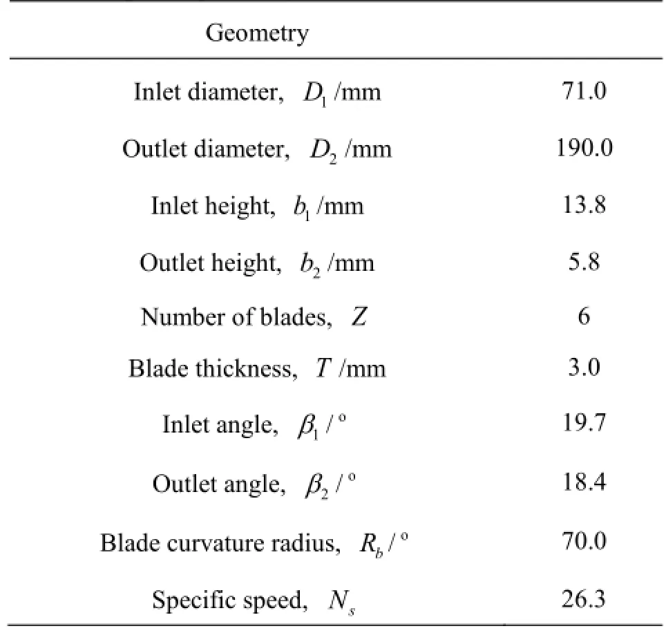
Table 1 Impeller geometry

The full passages of the impeller are simulated in the present work. To reduce the boundary influence, extensions are made at the outlet and the inlet of the flow passage, respectively. Due to the complexity of the computational domain, an unstructured hexahedron mesh is employed as it enjoys a good adaptability. In the near-wall regions, the mesh is refined according to the requirement of the LES. The grid stretching factor is selected to allow the wall-adjacent cells to be located within 0.02 mm of the surface corresponding tovalues, less than 5 near the wall, whereas the grids are also refined in the stream-wise and span-wise directions. A mesh of totally 2 381 970 cells is selected as the best adjustment between the solution accuracy requirements and the computer resources. Increasing the number of grids does not show a significant change of the results as shown by the grid independent test. Figure 2 represents the mesh construction of the full passage. The stretching factor near the wall is 1.1 and the value of the maximum aspect ratio is 218.

Fig.2 Computational grid

The rotation reference frame is adopted for the flow passage with the rotation speed being set to the rotation speed of the impeller. The inlet velocity boundary condition is determined by the flow rate, whichincludes some fluctuated velocity components normal to the inlet boundary. The Neumann conditionis adopted for the pressure. The value of the pressure is given at the outlet of the passage and the Neumann condition is taken into account for the velocity. Note that no-slip wall condition is adopted as

The time step is set as 0.00023 s that corresponds to a Courant number estimation of less than 10, i.e., overall 360 time steps per impeller revolution. The residual convergence criterion for each time step is reduced to 1.0×10-5, while the allowed maximum number of iterations per time step is limited to 15.

The introduced five SGS models are considered in the simulation and the calculated results are compared with the PIV and LDV experimental data taken from Ref.[20]. According to the standard error of the PIV data estimates and based on 1000 statistically uncorrelated samples, the statistical uncertainty in the mean velocities is set to 1.2. The statistical uncertainties in the LDV mean velocities are estimated to be 0.7%[20].

Fig.3 (Color online) Time-averaged velocity fields obtained by various SGS models

Fig.4 Radial and tangential velocities

3. Mean velocity field predicted

The following results are presented for the impeller mid-height. Figures.3(a)-3(e) show the time-averaged streamlines computed by using the SGS models and Fig.3(f) demonstrates the velocity vectors measured by the LDV. As shown in the LDV experiment, the blocked passage and the unblocked passage occur alternately in the impeller. This “two channel” phenomenon consisting of the alternated stalled and un-stalled passages, is captured by the DSM, the DMM and the DMNM, but not the SM and the DNM. The predictions are almost consistent with the measurement results, however an unreal small vortex is found for these three models in the blade suction of the un-stalled passage. This remarkable difference ismainly caused by the pre-rotation disregarded in the simulations[3]. According to the results, the size and the shape of the vortex computed by three models are different as the calculated vortex near the outlet obtained by the DMM is much smaller than those obtained by the other two models.

Fig.5 (Color online) Contour plots of the0.5)

In order to further examine the performance of the three SGS models in simulating the rotating stall phenomena, the radial and tangential velocities at theare compared for the points at the radial positions of(as shown in Fig.4). The velocity profiles at 0.25demonstrate a decent periodicity for every two passages within the full annulus. Therefore, only the results within a circumferential range ofare presented in the following sections, which contain two adjacent passages: A is the un-stalled passage, and B is the stalled passage. The results of the DNM and the SM are not presented in Fig.4 as these models fail to do the job. At0.5, the PIV measurements reveal that the velocity profiles in the passage A are skewed towards the suction side. However, all simulations predict velocity profiles that are displaced to the pressure side. This remarkable difference is mainly associated to the effects of pre-rotation[3]. According to Fig.4, in the passage B, the radial and tangential velocities illustrate a reversed flow along the suction side. The results of the DMNM and the DSM are in a decent agreement with the PIV results, however the DMM’s performance is not within the acceptable range. At, the performances of four models are almost the same in the passage A. Nevertheless in the passage B, the performance of the DMNM is in better agreement with the PIV results. At, all models appear to give predictions substantially deviated from the measurements of the radial velocity of the passage A. However, the predicted variation trend by the DMNM is in the best agreement with the experimental data. The tangential velocities of the passage B, predicted by the DMNM are in the best agreement with the PIV data. According to this detailed analysis of the models, the DMNM enjoys the highest accuracy in predicting the flow behavior.

4. Vorticity analysis

Figure 5 shows the time-averagedvorticity computed by using the SGS models. As shown in Fig.5(d), it presents the signi ficant strength of the inlet stall cell in passage B. According to this figure, avorticity of pronounced large magnitude is obtained across the inlet. Additional small clockwise rotating vortex is also observed to be shed from the pressure leading edge. It is clearly shown that thevorticity predicted by the DMM remarkably deviates from the measurements. Both the DMNM and the DSM have successfully captured small clockwise rotating vortices in the passage, however the size and the shape of the vortices still substantially deviate from the PIV results. Furthermore, the large value region in the DSM is larger than the region predicted by the DMNM and is more consistent with the PIV results.

5. Turbulence behavior analysis

Figure 6 illustrates the distribution of the twodimensional turbulent kinetic energyat the middle sectionof the impeller. This kinetic energy characterizes the extent of the instantaneous velocity deviation from the mean velocity, which is defined asNote thatu′ andare values of the instantaneous velocity rootmean square (rms) inplane. The stall phenomenon in passage B is associated with the high turbulence activity. Furthermore, the strong reversed flow from the vortex in the outlet region of the passage B gives rise to a signi ficant turbulence intensity. In the passage A, the DMM overestimates the turbulent kinetic energy. Also, a low value region is created near the entrance by using the DSM and the DMNM, which is in agreement with the PIV results. However, the DMM fails to predict such region. In the passage B, the DMM also gives an over-prediction at the passage entrance. In addition, the high value area predicted by the DSM has a lower value than the DMNM. The above explanations show that the predicted results by the DMNM are more consistent with the PIV results as compared to the results predicted by the other SGS models.

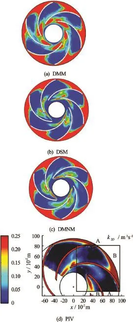
Fig.6 (Color online) Contours of the turbulent kinetic energy

In order to further evaluate the performance of the presented SGS models in the turbulence intensity prediction, the comparisons of the blade-to-blade distribution of the turbulence intensity are presented in Fig.7 at two radial positions, i.e.,and. According to this figure, atthe DMM over-predictsextensively as compared to PIV results. In the passage A, the DSM and the DMNM appear to be more reasonable, although both models predict profiles that are flatter than the PIV results due to the pre-rotation. In the passage B, the two models give the same peak magnitudes of the turbulent intensity in agreement with the PIV data. Nonetheless, when different positions are considered, the DMNM is more accurate than the DSM. Based on the results obtained atin the passage A, all predicted profiles for the turbulence intensity see higher values than the PIV results. Also, the models can not predict the peak value at the suction side. In the passage B, the DMNM and the DSM give results in a good agreement with the PIV results, unlike the DMM which gives a lower estimation of the turbulence intensity. Thus, it can be concluded that the twodimensional turbulent kinetic energy predicted by the DMNM is in the best agreement with the experimental values.

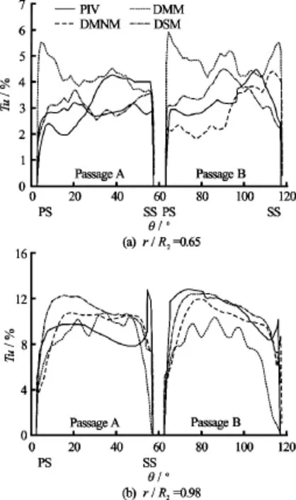
Fig.7 Turbulence intensity profiles

6. Conclusions

The internal flow in a shrouded six-bladed centri-fugal pump impeller under the stall condition is investigated in this paper by considering five different SGS models: SM, DSM, DNM, DMM and DMNM. The qualitative and quantitative comparisons are conducted between the simulation results and experimental tests.

Based on the results presented in this paper, the DMNM has great potentials to be used by pump designers to predict the flow performance under the stall condition of the pump.

[1] Luo X., Ji B., Tsujimoto Y. A review of cavitation in hydraulic machinery [J].Journal of Hydrodynamics, 2016, 28(3): 335-358.

[2] Zhou P. J., Wang F. J., Yao Z. F. Study on effects of blade number on stall characteristics for centrifugal pump impeller [J].Journal of Mechanical Engineering, 2016, 52(10): 207-215(in Chinese).

[3] Byskov R. K., Jacobsen C. B., Pedersen N. Flow in a centrifugal pump impeller at design and off-design conditions-Part II: Large eddy simulations [J].Journal of Fluids Engineering, 2003, 125(1): 73-83.

[4] Feng J., Benra F., Dohmen H. J. Application of different turbulence models in unsteady flow simulations of a radial diffuser pump [J].Forschung Im Ingenieurwesen, 2010, 74(3): 123-133.

[5] Lucius A., Brenner G. Numerical simulation and evaluation of velocity fluctuations during rotating stall of a centrifugal pump [J].Journal of Fluids Engineering, 2011, 133(8): 081102.

[6] Lucius A., Brenner G. Unsteady CFD simulations of a pump in part load conditions using scale-adaptive simulation [J].International Journal of Heat and Fluid Flow, 2010, 31(6): 1113-1118.

[7] Hasmatuchi V., Roth S., Botero F. et al. Hydrodynamics of a pump-turbine at off-design operating conditions: Numerical simulation [C].Proceeding of ASME-JSMEKSME Joint Fluids Engineering Conference. Shizuoka, Japan, 2011.

[8] Tao R., Xiao R., Yang W. et al. A comparative assessment of Spalart-Shur rotation/curvature correction in RANS simulations in a centrifugal pump impeller [J].Mathematical Problems in Engineering, 2014, 2014: 342905.

[9] Braun O. Part load flow in radial centrifugal pumps [D]. Doctoral Thesis, Lausanne, Switzerland: École Polytechnique Fédérale de Lausanne, 2009.

[10] Pacot O., Kato C., Avellan F. High-resolution LES of the rotating stall in a reduced scale model pump-turbine [C].27th IAHR Symposium on Hydraulic Machinery and Systems (IAHR 2014). Montreal, Canada, 2014.

[11] Kato C., Mukai H., Manabe A. Large-eddy simulation of unsteady flow in a mixed-flow pump [J].International Journal of Rotating Machinery, 2003, 9(5): 345-351.

[12] Posa A., Lippolis A., Verzicco R. et al. Large-eddy simulations in mixed-flow pumps using an immersed-boundary method [J].Computers and Fluids, 2011, 47(1): 33-43.

[13] Yang Z., Wang F., Zhou P. Evaluation of subgrid-scale models in large-eddy simulations of turbulent flow in a centrifugal pump impeller [J].Chinese Journal of Mechanical Engineering, 2012, 25(5): 911-918.

[14] Yang Z., Wang F. A dynamic mixed nonlinear subgridscale model for large-eddy simulation [J].Engineering Computations, 2012, 29(7): 778-791.

[15] Smagorinsky J. General circulation experiments with the primitive equations [J].Monthly Weather Review, 1963, 91(3): 99-164.

[16] Ryu S., Iaccarino G. A subgrid-scale eddy-viscosity model based on the volumetric strain-stretching [J].Physics of Fluids, 2014, 26(6): 065107.

[17] Vollant A, Balarac G., Corre C. A dynamic regularized gradient model of the subgrid-scale stress tensor for largeeddy simulation [J].Physics of Fluids, 2016, 28(2): 025114.

[18] Singh S., You D. A dynamic global-coefficient mixed subgrid-scale model for large-eddy simulation of turbulent flows [J].International Journal of Heat and Fluid Flow, 2013, 42: 94-104.

[19] Yang Z., Cui G., Xu C. et al. Large eddy simulation of rotating turbulent channel flow with a new dynamic globalcoefficient nonlinear subgrid stress model [J].Journal of Turbulence, 2012, 13(48):1-20.

[20] Pedersen N., Larsen P. S., Jacobsen C. B. Flow in a centrifugal pump impeller at design and off-design conditions−Part I: Particle image velocimetry (PIV) and laser doppler velocimetry (LDV) measurements [J].Journal of Fluids Engineering, 2003, 125(1): 61-72.

(Received December 30, 2014, Revised June 30, 2015)

* Project supported by the National Nature Science Foundation of China (Grant Nos. 51139007, 51321001), the Natural Science Foundation of Zhejiang Province (Grant No. LQ17E090005) and the National Science and Technology

Support Program of China (Grant No. 2015BAD20B01).

Biography: Pei-jian Zhou (1986-), Male, Ph. D.

Fu-jun Wang,

E-mail:wangfj@cau.edu.cn