Y. Luo, C. N. Kim, M. Q. Zhu

1.Department of Mechanical Engineering, Graduate School, Kyung Hee University, Yong-in, Korea,

E-mail: 329971597@qq.com

2.Department of Mechanical Engineering, College of Engineering, Kyung Hee University, Yong-in, Korea

Magnetohydrodynamic flows tuning in a conduit with multiple channels under a magnetic field applied perpendicular to the plane of flow＊

Y. Luo1, C. N. Kim2, M. Q. Zhu1

1.Department of Mechanical Engineering, Graduate School, Kyung Hee University, Yong-in, Korea,

E-mail: 329971597@qq.com

2.Department of Mechanical Engineering, College of Engineering, Kyung Hee University, Yong-in, Korea

In this study, three-dimensional liquid-metal magnetohydrodynamic flows in a conduit with multiple channels under a uniform magnetic field are numerically investigated. The geometry of the conduit is of a four-parallel-channels system including one inflow channel and three outflow channels. The liquid-metal flows into the inflow channel, then turns throughin the transition segment, finally flows into three different outflow channels. This kind of channel system can induce counter flow and co-flow, which is rarely investigated before though the conceptual designs of duct flow in the blanket have suggested this type of flow. A structured grid system is chosen after a series of mesh independence tests in the present study. The axial velocity in the side layer near the first partitioning wall, located between the inflow channel and the first outflow channel, is the highest with the lowest electric potential formed therein. The pressure almost linearly decreases in the main flow direction, except in the transition segment. Moreover, the pressure gradient in the first outflow channel is the largest among the three outflow channels. The interdependency of the current, fluid velocity, pressure, electric potential is examined in order to describe the electromagnetic characteristics of the liquid-metal flows.

Liquid-metal, magnetohydrodynamics, multiple channels

Introduction

This study explores the flow of an electrically conducting fluid under an external magnetic field. Magnetohydrodynamic (MHD) flow is a field of great interest in engineering applications, especially important in the design of liquid-metal (LM) cooling system of fusion reactor, where a plasma is confined by a strong magnetic field[1]. The fluid motion of LM in a strong magnetic field results in serious MHD effects, having enormous impact on velocity distribution, pressure drop and the required pumping power for the cooling system[2]. Therefore, the knowledge of LM MHD flow characteristics is one of the key issues in the optimal design for LM blanket.

A number of experimental studies have been conducted to investigate the LM MHD effects. Bühler et al.[3]performed experiments to investigate the LM flows through a sudden expansion of rectangular ducts at high Hartmann numbers. Stieglitz et al.[4]experimentally investigated the MHD flow in a direction perpendicular to the magnetic field.

A mathematical approach[5,6]has been taken to analyze the velocity profile in the developed region. Siddheshwar and Mahabaleswar[7]used mathematical method to study the MHD flow in a viscoelastic liquid. To make the analysis of MHD flow easier, numerous theoretical studies on MHD flow have been performed with an inertialess approximation. The asymptotic techniques[8]on MHD flows can be used, when the flow is fully developed or when the value of the interaction parameter is extremely large. Walker and Ludford[9]employed asymptotic techniques to analyze MHD flows in rectangular ducts with variable cross-sectional areas. However, the inertial effects cannot always be negligible in flows where liquid metal flows in complicated conduits, especially when the ratio of the interaction parameter to the Hartmann number is small[10]. For the complex geometries offlow channels in blankets, detailed investigation of MHD flow characteristics is difficult with the use of theoretical analysis.

Fig.1 Duct geometry, coordinate system and the magnetic field applied (mm)

With the development of computer science, the numerical simulation becomes an effective method for analyzing MHD effects and optimizing blanket design. A lot of numerical codes have been developed for investigating liquid metal MHD flows. Vantieghem et al.[11]numerically investigated the velocity profile of laminar MHD flows in circular conducting pipes using a finite-volume code with high resolution unstructured meshes. Madarame and Tokoh[12]built a code that could analyze the MHD flows in a semi-cylindrical pipe under a uniform magnetic field.

In addition, three-dimensional numerical works with the use of CFX code have been employed for MHD flows in complex duct geometries. Reimann et al.[13]assessed pressure drop and velocity distribution in their study in which a strong three-dimensional electric current occurs, and explained the multi-channel effects in LM MHD duct flows. In the manifold with three sub-channels of co-current flow, the fully developed velocity profiles were numerically obtained with CFX software. However, there are no detailed explanations of the specific conditions for the MHD flow. Arshad et al.[14]performed a detailed numerical study of LM flow in a curved bend under two kinds of magnetic fields. The MHD pressure drop increases as the liquid metal flows increasingly transverse to the magnetic field. Morley et al.[15]performed a numerical simulation of MHD flows in a geometry consisting of a single rectangular duct and three rectangular subchannels that are perpendicular to the applied magnetic field.

Although many studies on MHD flows in complicated geometries have been recently performed, the LM MHD flows in a conduit with multiple channels under a uniform magnetic field have rarely been investigated in detail before. This study numerically analyzes the three-dimensional MHD flows in a conduit with parallel inflow and outflow channels under a uniform magnetic field perpendicular to the plane of the flow. Here, the cooled liquid metal flows into the blanket through an inflow channel, reaches the region near the first wall, and comes back through the multiple outflow channels, resulting in co-flows and counter-flows. This type of flow system can be one of the good candidates for the flow design for the purpose of cooling the first wall and blankets. If the characteristics of MHD flows in the present study are to be investigated successfully, the results can be used to design the flows system with higher efficiency of heat extraction. Therefore, it is highly meaningful to examine the features of the proposed flows. In order todescribe the electromagnetic characteristics of the LM MHD flows, the interdependency of the current, fluid velocity, pressure and electric potential is examined, and the detailed information about these flow variables is discussed with different Hartmann numbers, different conductance ratios and different geometries.

1. Problem formulation and solution method

1.1Geometry, magnetic field and materials

This study investigates three-dimensional liquidmetal MHD flows in a conduit with multiple channels. The geometry of the conduit is shown in Fig.1. Applied in thez-direction is the uniform magnetic fieldscorresponding to Hartmann number 1 000, 600 and 300 in different cases, respectively. The Hartmann number and conductance ratio can be defined as follows:

Hartmann number

Table 2 Cases with different Hartmann numbers and different conductance ratios

1.2Governing equations

A steady-state, incompressible, constant-property, laminar flow of an electrically-conducting liquid metal under the influence of an external magnetic field is governed by the following equations:

Conservation of mass

Equation of motion

Conservation of the charge

Fig.2 (Color online) Current density and electric potential in theplane atin Case 1-1

Substituting Eq.(6) into Eq.(5) gives the electrical potential Poisson equation as

This means that the equation of mass conservation and the equation of motion can be solved together with Eq.(7) for the variables of the pressure, velocity, and electrical potential in the fluid region. In addition, because the velocity of the solid region is zero, only Eq.(7) is used for the electric potential in solid parts with

1.3Boundary conditions

No slip condition is applied at the fluid-solid interface. At the inlet a uniform velocityis given, and at the outlets there is no change in the variable (except for the pressure) in the main flow direction. Since the change of pressure is meaningful in the flow domain, the pressure value can be considered to be zero at the outlets. For the boundary condition of the electric potential, it is considered that the whole system including the fluid and walls are electrically insulated from the outside.

1.4Numerical method

The present study uses a structured grid system with 4 603 890 grids after a series of grid independence tests. Finer grids are employed in the fluid region near the walls and in the transition segment. In all cases, three cells in the Hartmann layer and twenty five cells in the side layer are used, respectively. Underrelaxation is utilized in the iteration procedure for the coupled governing equations. The second-order upwind scheme is used to discretize the convective terms and the central difference scheme for diffusion terms.

Fig.3 (Color online) Schematic of plane current in theplane atin Case 1-1

Fig.4 (Color online) Distribution of the axial velocity in theplane atin Case 1-1

Fig.5 (Color online) Current density and electric potential in theplane atin Case 1-1

Fig.6 (Color online) Schematic of plane current in theplane at(near the end of the partitioning wall) in Case 1-1

A multigrid-accelerated Incomplete Lower Upper Factorization technique[16]is employed. For the pressure-velocity coupling Rhie-Chow Interpolation method[17]is used. For the validation of the current numerical modeling with the use of CFX code, a numerical study[18]can be referred to.

2. Results and discussions

In this study, three different cases with different conductance ratios are considered. And, in each case three different subcases with different Hartmann number are examined (Table 2).

2.1Case 1-1

In the present study, the components on the right side of the general Ohmʼs law (Eq.(6)) are distinguished in order to describe the independency of the flow variables. Therefore,can be expressed by. The firstdenotes the current induced by the electric field, and it can be named the electric-field component of the current (EFCC). The second term,, means the current induced by the fluid motion in a magnetic field, and it can be referred to as the electro-motive component of the current (EMCC).

The characteristics of the flow field are examined in several local regions (that is, in the inflow channel, in the transition segment and in the outflow channels). Figure 2 shows the distributions of the current density and electric potential in theplane at(the half-length of the partitioning wall). In Fig.2, since the main flow in the inflow channel is indirection and the magnetic field is applied indirection, the current flow in the negativedirection is induced in the fluid region. Then, the current returns to the first partitioning wall through the duct walls. However, in the outflow channels, the current flows upward in the fluid region, then comes back to the first partitioning wall through the duct walls. More specifically, in the inflow and in the first outflow channel, the current in the fluid region near the first partitioning wall converges to the central part of the fluid region because the vector summation of the EMCC and EFCC yields the obliquely downward and upward current, respectively (see also Fig.3). The current moves upward in the fluid region above the first partitioning wall, while the current moves downward in the region below the first partitioning wall. So, the electric potential on the first partitioning wall (and in the fluid region near the first partitioning wall) is the lowest, with the formation of high electric potential in the fluid region near the bottom and top walls. Here, it is to be reminded that the current flow and electric potential have mutual influence on each other.

Figure 3 shows a schematic of the plane current in theplane at. In the inflow channel the current moves downward, and in the three outflow channels the current moves upward as shown in Fig.2. Since the EMCC is induced by the fluid motion and the EFCC is created by the electric field, in association with the distribution of electric potential shown in Fig.2 the vector summation of the EMCC and EFCC can yield obliquely upward and downward current in the fluid region near the top wall, bottom wall, and the first partitioning wall, respectively.

Figure 4 shows the distribution of the axial velocity in theplane at. The velocities in the regions near the first partitioning wall (especially, in the inflow channel) and the bottom wall are higher, which is caused by the smallercomponent of current density therein (see Fig.3). Notice that the axial velocity in the side layer below the first partitioning wall (in the inflow channel) is the highest. Moreover, the lowest axial velocity (this means the highest negativevelocity) is observed in the fluid region above the first partitioning wall (in the first outflow channel).

The distributions of the current density and electric potential in theplane at(in the cross-section near the end of the partitioning walls) are shown in Fig.5. In the inflow channel, the current heads downward, then returns to the first partitioning wall through the duct walls. In the outflow channels, the current moves upward. However, in the first outflow channel, the current distribution is more complex because of the complicated velocity therein. In the lower part of the first outflow channel, the current converges to the central part of the fluid region because of the existence of a region with low electric potential above the end of the first partitioning wall (see also Fig.10). As can be expected, higher electric potential is formed on the top wall (and in the fluid region near the top wall-fluid interface) and on the bottom wall (and in the fluid region near the bottom wall-fluid interface), while the much lower electric potential is induced on the first partitioning wall and in the fluidregion near the first partitioning wall. Here, the electric potential value of the central point of the top and bottom wall is 0.000319 V and 0.000325 V, respectively. The lowest value of electric potential (−0.000327 V) is observed in the central point of the first partitioning wall.

Fig.7 (Color online) Plot of thecomponents of velocity in theplane atin Case 1-1

Fig.8 (Color online) Current density and electric potential in theplane atin Case 1-1

Fig.9 (Color online) Plane velocity in the midplane atnear the transition segment in Case 1-1

Figure 6 presents a schematic of the plane current in theplane at. In the inflow and outflow channels, the EMCC is larger than the EFCC, so that the current is induced to head downward in the inflow channel, and to move upward in the outflow channel, respectively. In the lower part of the first outflow channel, the current converges to the midplane with considerable EFCC therein. In the fluid region near the partitioning walls (in the three outflow channels) and top wall, the obliquely upward current is induced by the vector summation of the EMCC and EFCC. In the fluid region near the first partitioning wall (in the inflow channel) and the bottom wall, the current moves obliquely downward. Notice that, in each of the fluid region below the second and third partitioning walls (in the first and second outflow channels, respectively), the EMCC is headed downward because of the positivevelocity therein (see also in Fig.9).

Figure 7 shows the distribution ofcomponents of velocity in theplane at. The positivevelocity is observed in the whole region of inflow channel and in some parts of the fluid regions below the second and third portioning walls.High velocity is observed in the side layers (near the partitioning and bottom walls) of the inflow channel (see Fig.7(a)). Figure 7(b) shows the distribution of negativecomponent of velocity, where the lowest axial velocity is formed in the fluid region above the first partitioning wall. As expected, in the fluid region very near the first partitioning wall (in the inflow channel), the highest velocity is formed (see also in Fig.7(c)).

The distributions of the current density and electric potential in theplane at(in the transition segment) are display in Fig.8. In the lower part of the transition segment, the current flows downward, while in the upper part of the transition segment, the current flows upward. As can be seen in Fig.8, higher electric potential is formed near the top and bottom walls, while lower electric potential is observed in the fluid region above the end of the first partitioning wall. The electric potential value of the central point of the bottom and top wall is 0.000305 V and 0.000297 V, respectively. The lowest electric potential value is 0.000131 V.

Fig.10 (Color online) Electromagnetic features in the midplane atin Case 1-1

Figure 9 shows the velocity distribution in the midplane atin a region including the transition segment. Before entering the transition segment, the fluid flows in the positivedirection, with higher velocity in the side layer near the first partitioning wall and bottom wall. In the transition segment, the highest velocity is observed in fluid region near the end of the first partitioning wall (Fig.9(a)). The positivecomponent of velocity is observed under the end of the second and third partitioning walls, as shown in Figs.9(b) and 9(c). The separated flow yields the velocity recirculation above the end of the partitioning walls. This kind of velocity pattern makes each of the end of partitioning walls have lower electric potential. Moreover, the velocity recirculation above the end of the first partitioning wall is largest, thus the lowest electric potential is observed therein (see also Fig.10(a)). Since the magnetic field is applied indirection, the flow indirection at the bottom of the transition segment induces the EMCC in the negativedirection, and the flow indirection in the middle of the transition segment created the EMCC in thedirection. Also, the flow in negativedirection at the top of the transition segment yields the EMCC in thedirection, which results in the higher electric potential in the regions near the bottom wall, end wall, and top wall.

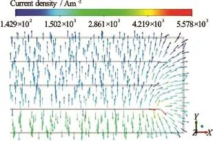
Fig.11 (Color online) Current density in the midplane atnear the transition segment in Case 1-1

The distribution of the electric potential in the midplane including the transition segment is presented in Fig.10(a). In association with the direction of the EMCC, a higher electric potential is induced oin the outer walls (and in fluid regions very near the outer walls). The recirculating flows observed just above the tip of each partitioning wall (Figs.9(b)-9(d)) leads to the lower electric potential at the end of each partitioning wall. More specifically, the lowest electric potential is observed near and above the end of the first partitioning wall because of the upward highest velocity and the largest velocity recirculation therein as shown in Fig.10(b), which presents the schematics of the current flow in the region of flow separationnear the end of the first partitioning wall. In fluid region moderately above and right to the region of the lowest electric potential (see Fig.10(b)), the EMCC (denoted by) is quite larger than the EFCC (expressed by) because of higher velocity therein. However, in the fluid region just above, and near, the end of first partitioning wall, the EMCC (caused by velocity indirection therein) is weaker than the EFCC (caused by the spatial change in the electric potential), which yields the current in an obliquely upward direction (see Fig.11) in the fluid region including the tips of partitioning walls.

Figure 11 shows the current density in the midplane near the transition segment. In the inflow channel, the current flows in the downward direction. In the transition segment, the current flows radially from the end of the first partitioning wall to the outer walls, as explained before.

Fig.12 (Color online) The distributions ofdirectional velocity component in theplane at,and in theplane atin Case 1-1

Figure 12 depicts the distribution of thecomponent of velocity in the three planes which are close to the fluid-wall interface in Case 1-1. As shown in Fig.12(a), the twoplanes are located at0.006 m and(named the outerplanes), while theplane is located at1.619 m (named the outerplane). Firstly, four rugby ball-shaped regions of thecomponent of the velocity are formed, which are pairwise-symmetric with respect to the edge line of the right angle (or, point symmetric with respect to themed point of the corner). In the bottom side layer of the inflow channel flow, the axial velocity diverges in theplane, yielding positive and negativecomponent of velocity (before the first turning of the main flow, as shown in Fig.12(b)). After turning, in the outerplane the velocities converge to the central fluid region. Also, in the upper part of outerplane, the velocity in this plane undertakes the same flow pattern so that before the second turning, in the outerplane the velocities diverge, and after the second turning, the velocities converge to the central region. This type of phenomen on is believed to be related to local change in current density.

The axial velocities (absolute value) in the inflow and outflow channels in theplane atare obtained, yielding “M-shape” velocity profiles, as shown in Fig.13. In the outflow channels, the axial velocity near the first partitioning wall is larger than that near the second and third partitioning walls. Moreover, the axial velocity in the fluid region below the first partitioning wall (in the inflow channel) is larger than that in the fluid region above the first partitioning wall (in the first outflow channel).

Fig.13 (Color online) Axial velocity distributions (absolute value) in the cross-section atin Case 1-1

Fig.14 (Color online) Pressure distributions in Case 1-1 and Case 4

2.2Case 4 with a different geometry and the comparison of the Cases

In order to examine the effect of the geometric features on the pressure distribution, a multiple channel system with one inflow channel and two outflow channels is considered in Case 4 where the Hartmann number and conductance ratio are the same as those in Case 1-1. Figure 14 depicts the distribution of the pressure in Case 1-1 and Case 4. In both cases, the pressure almost linearly decreases in the main flow direction. As can be seen in Fig.14(a), the pressure in the inflow channel decreases more rapidly than that in any of outflow channels, implying the highest pressure gradient because the current flowing in the fluid region has the shortest length of the electric current loop through the duct wall with the least electric resistance association with this electric current loop. Moreover, the pressure gradient of the first outflow channel is the largest among the outflow channels. Figure 14(b) shows the pressure distribution in the segment region, where the pressure gradient of lower part of the segment region (the line BC of Case 1-1 and the line JK of Case 4) is the largest in the transition segments in the two cases. However, there are some difference in pressure gradient in the inflow and outflow channel between Case 1-1 and Case 4. The pressure gradient in the inflow channel of Case 1-1 is slightly larger than that in Case 4, while the pressure gradients in the outflow channels and segment region of Case 1-1 are fairly smaller than those in Case 4.

Table 3 Mass flow rates in cases with different Hartmann numbers and different conductance ratios

Table 4 Mass flow rates in two cases with different geometries

Here, the non-dimensional pressure gradientsof the four sub-channels in the region (for) in Case 1-1 are evaluated to be 0.526 (inflow channel), 0.499 (first outflow channel), 0.516 (second outflow channel), 0.527 (third outflow channel), respectively. In the region (for), the non-dimensional pressure gradients of the three sub-channels in Case 4 are evaluated to be 0.526 (inflow channel), 0.513 (first outflow channel) and 0.528 (second outflow channel), respectively.

The effect of the Hartmann number and conductance ratio on the distribution of mass flow rate in the three-outflow channels in Case 1, Case 2, and Case 3 (see Table 2) is investigated. Table 3 shows the mass flow rate in different cases (with different Hartmann numbers and different conductance ratios). As the Hartmann number increases (with a fixed conductance ratio), the mass flow rate in the first outflow channel increases, while that in the second and third outflow channels decrease. In all cases, the mass flow rate in the first and third outflow channels are relatively higher than that in the second outflow channel, showing a meaningful imbalance in the mass flow rate. The differences in the mass flow rate among the three outflow channels are smaller when the Hartmann number is smaller. With a fixed Hartmann number, when the conductance ratio is the smallest, the mass flow rate of the first outflow channel and the difference in the mass flow rate between the first and second outflow channels are the smallest.

Table 4 shows the comparison of mass flow rate in Case 1-1 and Case 4. Among each outflow channel of Case 1-1 and Case 4, the largest mass flow rate is observed in the first outflow channel. The difference in the mass flow rate between the first and second outflow channels in Case 1-1 is larger than that in Case 4.

3. Conclusions

This study numerically investigates the threedimensional LM MHD flows in a conduit with multiple channels in the plane perpendicular to a uniform magnetic field using CFX. The detailed features of LM MHD flow are predicted in terms of flow velocity, current, electric potential and pressure distributions.

For the LM MHD flows in a conduit system with four sub-channels (one inflow channel and three outflow channels), case study with different Hartmann numbers and different conductance ratios is carried out. The simulation results of the case (the Hartmann number is 1 000 and the conductance ratio is 0.541) show that the axial velocity in the side layer near the first partitioning wall is higher than that near the outer walls. And, in the inflow and outflow channels obtained are the “M-shape” velocity profiles. A lowerelectric potential is observed near the first partitioning wall, while a higher electric potential is induced near the outer walls. In the transition segment, the separated flow yields complicated distributions of the electric potential and current therein, and a large vortex is formed at the entrance of the first outflow channel (above the end of the first partitioning wall). Moreover, for the mass flow rate in the conduit with four sub-channels, when the conductance ratio is fixed, the mass flow rate in the first outflow channel increases, while that in the second and third outflow channels decreases with the increase of the Hartmann number. For a fixed Hartmann number, when the conductance ratio is the smallest, the mass flow rate of the first outflow channel is the smallest. Also, the pressure distributions in two cases with different geometries are investigated. One case is the conduit with four sub-channels (one inflow channel and three outflow channels), and another case is the conduit with three sub-channels (one inflow channel and two outflow channels). In both cases, the pressure almost linearly decreases in the main flow direction, except in the transition segment.

In summary, this study investigates the electromagnetic features of LM MHD flows in a conduit with multiple channels in cases with different Hartmann numbers, different conductance ratios and different geometries. Two components of the current (i.e.,in Ohmʼs law are separately considered to explain the independency among the fluid velocity, current, and the electric potential. The imbalance of the mass flow rate is affected by the Hartmann number, the conductance ratio and the geometric feature of the conduit.

Acknowledgements

This work was supported by National R&D Program through the National Research Foundation of Korea (NRF) funded by the Ministry of Education, Science and Technology and Ministry of knowledge Economy (Grant No. 2015M1A7A1A02050613).

[1] Mistrangelo C., Buhler L. Numerical investigated of liquid metal flows in rectangular sudden expansions [J].Fusion Engineering and Design, 2007, 82(15-24): 2176-2182.

[2] Zhou T., Yang Z., Ni M. et al. Code development and validation for analyzing liquid metal MHD flow in rectangular ducts [J].Fusion Engineering and Design, 2010, 85(10-12): 1736-1741.

[3] Bühler L., Horanyi S., Arbogast E. Experimental investigation of liquid-metal flows through a sudden expansion at fusion-relevant Hartmann numbers [J].Fusion Engineering and Design, 2007, 82(15-24): 2239-2245.

[4] Stieglitz R., Barleon L., BüHler L. et al. Magnetohydrodynamic flow through a right-angle bend in a strong magnetic field [J].Journal of Fluid Mechanics, 1996, 326: 91-123.

[5] Hunt J. C. R., Shercliff J. A. Magnetohydrodynamics at high Hartmann numbers [J].Annual Review of Fluid Mechanics, 1971, 3: 37-62.

[6] Hunt J. C. R. Magnetohydrodynamic flow in rectangular ducts [J].Journal of Fluid Mechanics, 1965, 21(4): 577-590.

[7] Siddheshwar P. G., Mahabaleswar U. S. Effects of radiation and heat source on MHD flow of a viscoelastic liquid and heat transfer over a stretching sheet [J].International Journal of Non-Linear Mechanics, 2005, 40(6): 807-820.

[8] Sommeria J., Moreau R. Why, how, and when, MHD turbulence becomes two-dimensional [J].Journal of Fluid Mechanics, 1982, 118: 507-518.

[9] Walker J. S., Ludford G. S. S. MHD flows in conducting circular expansions with strong transverse magnetic fields [J].International Journal of Engineering Science, 1974, 12(3): 193-204.

[10] Umeda N., Takahashi M. Numerical analysis for heat transfer enhancement of a lithium flow under a transverse magnetic field [J].Fusion Engineering and Design, 2000, 51-52: 899-907.

[11] Vantieghem S., Albets-Chico X., Knaepen B. The velocity profile of laminar MHD flows in circular conducting pipes [J].Theoretical and computational fluid dynamics, 2009, 23(6): 525-533.

[12] Madarame H., Tokoh H. Development of computer code for analyzing liquid metal MHD flow in fusion reactor blankets [J].Journal of Nuclear Science and Technology, 1988, 25(3): 233-244.

[13] Reiman J., Buhler L., Mistrangelo C. et al. Magnetohydrodynamic issues of the HCLL blanket [J].Fusion Engineering and Design, 2006, 81(1-7): 625-629.

[14] Arshad K., Majid A., Rafique M. et al. Numerical simulation of magnetohydrodynamic pressure drop in a curved bend under different conditions [J].Fusion engineering and design, 2007, 18(1): 1-12.

[15] Morley N. B., Ni M. J., Munipalli R. et al. MHD simulation of liquid metal flow through a toroidally oriented manifold [J].Fusion Engineering and Design, 2008, 83(7-9): 1335-1339.

[16] Raw M. Robustness of coupled algebraic multigrid for the Navier-Stokes equations[C].AIAA 34th Aerospace Science Meeting and Exhibit. Reno, USA, 1996, 96-0297.

[17] Shen W. Z., Michelsen J. A., Sorensen J. N. Improved Rhie-Chow interpolation for unsteady flow computations [J].AIAA Journal, 2001, 39(12): 2406-2409.

[18] Kim C. N. Magnetohydrodynamic flows entering the region of a flow channel insert in a duct [J].Fusion Engineering and Design, 2014, 89(1): 56-68.

(Received May 31, 2015, Revised December 1, 2015)

* Biography: Y. Luo (1991-), Female, Ph. D. Candidate

C. N. Kim, E-mail: cnkim@khu.ac.kr