Pei-jian Zhou （周佩剑）, Jia-cheng Dai（戴嘉铖）, Ya-fei Li（李亚飞）, Ting Chen（陈婷）,Jie-gang Mou （牟介刚）

1. College of Mechanical Engineering, Zhejiang University of Technology, Hangzhou 310034, China

2. Engineering Research Center of Process Equipment and Remanufacturing, Ministry of Education, Hangzhou 310034, China

3. School of Science, Wuhan Institute of Technology, Wuhan 430205, China

Abstract: The stall is an unsteady flow phenomenon that always causes instabilities and low efficiency for pumps. This paper focuses on the unsteady flow structures and evolutions under two types of stall conditions in centrifugal pump impellers. Two centrifugal pump impellers, one with 6 and another with 5 blades, are considered and a developed large-eddy simulation method is adopted. The results show that the alternative stall occurs in the impeller with 6 blades, while, the rotating stall is observed in that with 5 blades. The flow structure and the pressure fluctuation characteristics are further analyzed. For the alternative stall, the stall cells are fixed relative to the impeller, but a large vortex in the stalled passage is always swaying. The outlet vortex is generated from it, and then develops and sheds periodically. For the rotating stall, the stall cells first occur in the suction side of the blade. With the growth of the stall cells, the block area gradually increases until the inlet region is almost blocked, then moves to the pressure side with a continuous decay. When the rotating stall occurs, the amplitude of the pressure fluctuation is much larger than that under the alternative stall condition. The propagation of the stall cells has a significant effect on the pressure fluctuations in the impeller.

Key words: Centrifugal pump, flow structures, rotating stall, alternative stall, large-eddy simulation

Introduction

The stall is an unsteady flow phenomenon that always causes instabilities and low efficiency for pumps[1-4]. Under the stall condition, the periodic generation and shedding of the stall cells always induce significant low frequency pressure fluctuations and vibrations, with a severe influence on the safety and stability of pumps. It is necessary to study the stall phenomenon to improve the safety and the stability of the pump operation. This study focuses on the unsteady flow structures and evolutions under two types of stall conditions in the centrifugal pump impellers.

The stall, as an unsteady flow phenomenon,occurs in pumps due to the flow separation along the flow-guiding parts[5]. The large region of the separated flow is considered as the stall cell, which plays an important role in pumps, and can induce vibrations,noises, and even severe damages to the machine[6-7].Therefore the characteristics of the stall cells are important factors in improving not only the efficiency but also the operating safety and stability of pumps.

So far, only a few experimental studies are found in literature for the stall phenomenon in centrifugal pumps. Pedersen et al.[8]used the particle image velocimetry (PIV) to show the internal flow through a centrifugal pump impeller, and identified the alternative stall for the first time. Further investigations were followed, including the study performed by Johnson et al.[9], which showed that these stall patterns also existed in the volute pump. Feng et al.[10], Ullum et al.[11]found similar stall cells in the vaned centrifugal pumps. Krause et al.[12]adopted the time-resolved PIV to find another type of stall called the rotating stall, where the instabilities occurred at a low flow rate. However, the PIV has some limitations,such as in the time resolution and the measurement area. Thanks to the development of the computational fluid dynamics (CFD), the stalled flows in the centrifugal pumps were numerically studied. Feng et al.[13]applied different turbulence models for unsteady flow simulations of a radial diffuser pump, and the results showed that the RANS models often failed to predict the stall phenomenon. The SST -kω model could capture the stall cells, but with a large deviation when the stall occurred[14]. The large-eddy simulation(LES) shows a promising advance for complex turbulent flows. A series of validation simulations are performed for the stall phenomenon, and the results are in an excellent agreement with the available experimental data[5,15].

In the above studies, the stall phenomena were identified in centrifugal pumps. However, the structures and the motion of the stall cells are not yet fully understood. This study focuses on the stall cell characteristics in a centrifugal pump impeller by analyzing two types of stall phenomenon. The flow field and the stall cell structures are represented based on a developed large-eddy simulation with the dynamic mixed nonlinear model (DMNM).

1. The investigated pump and simulation details

The investigated pump impeller is a shrouded,low specific-speed centrifugal impeller with 6 blades,as shown in Fig. 1. Under the design condition, the pump flow rate is=3. 0 6 L/ s and the head is=1.75 m. More detailed geometric and experimental data can be found in Ref. [8]. In order to study two types of stall phenomenon, another one with 5 blades is considered in the study, with the otherwise same geometry. The large-eddy simulation is performed under the initial stall condition, the developed stall conditionand the deep stall condition

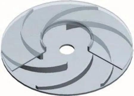
Fig. 1 Geometry of the impeller with 6 blades

The entire flow passages of the impeller is modelled and simulated. In order to reduce the boundary influence, extensions are made at the outlet and the inlet of the flow passage, respectively. Owing to the complexity of the computational domain, the unstructured hexahedron mesh is employed because of its fine adaptability. In the near-wall region the mesh is refined according to the requirement of the LES. In view of the Ref. [16] the grid stretching factor is chosen to allow the wall-adjacent cells to be located 0.02 mm off the wall, whilst also refining the grids in the streamwise and spanwise directions. A mesh of a total 3.2×106cells is utilized as the best compromise between the solution accuracy requirements and the available computer resources. Increasing the number of grids does not make a significant difference during the grid independent process. Figure 2 represents the mesh construction of the full passages.

Fig. 2 Computational domain and mesh

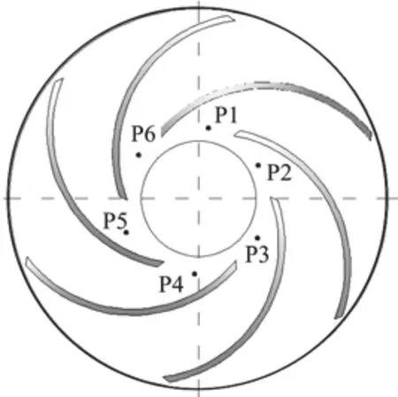
Fig. 3 The locations of monitor points

A rotational reference frame is set for the flow passage, with the rotating speed of the reference frame equal to the rotating speed of the impeller. The velocity inlet boundary condition is chosen in the simulation. The inlet velocity is determined by the flow rate, including some fluctuation components,with the velocity normal to the inlet boundary. The Neumann condition, ∂φ/∂n=0, is considered for the pressure. At the outlet of the passage the pressure is given. The no-slip wall condition is considered, as u =0, v = 0, w = 0.

The time step is set as 0.00023 s corresponding to a Courant number estimation smaller than 10, with a total 360 time steps per impeller revolution. The residual convergence criterion for each time step is reduced to 10-5, while the maximum number of iterations allowed per time step is limited to 15.

The arrangement of the recording points is shown in Fig. 3. In view of the prediction for the number and the speed of the stall cells, the monitor points (P1-P6)are uniformly distributed on the shroud of the impeller for recording the pressure fluctuations.

A developed large-eddy simulation with the dynamic mixed nonlinear model (DMNM) is performed on a full annulus of the impeller. The key to the success of the LES is to accurately represent the subgrid-scale (SGS) stress. The SGS stress can be written as follows[17]

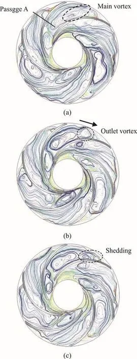
Fig. 4 (Color online) Evolution of outlet vortices

In the DMNM, the resolved modified Leonard term and the modelled modified cross term are retained, with the modified Reynolds stress. This model combines the advantages of the dynamic mixed model (DMM) and the dynamic nonlinear model(DNM). The previous work shows that the DMNM,with its inclusion of the turbulent anisotropic properties, is more suitable for high curvature, strong rotational turbulence calculations[18]. The derivation details of this model can be found in the Ref. [19].

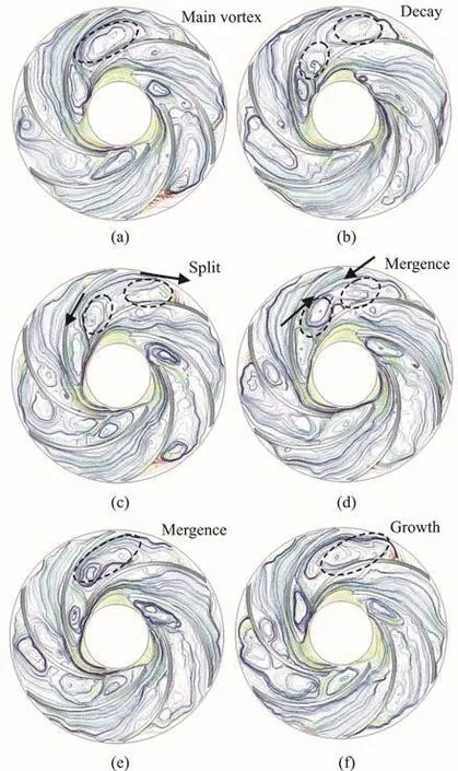
Fig. 5 (Color online) Evolution of main vortices

2. Alternative stall

2.1 Flow structures analysis

The alternative stall occurs in the impeller with 6 blades. As shown in Fig. 4, the stalled and unstalled passages can be observed, as reported by Pedersen et al.[8]. Three stall cells block the entrance of the passage, which does not rotate with respect to the impeller. Besides, one observes another two types of vortex motion in the stalled passage. The passage A is taken as an example to analyze the flow structures. A larger vortex appears downstream, which is more unsteady with characteristics of the wake flow due to the adverse pressure gradient and the centrifugal force.As the flow develops, the large vortex shakes and splits into small vortexes at the passage outlet. Then,the main vortex core gradually moves downstream,induces the shedding of the outlet vortex and disappears.

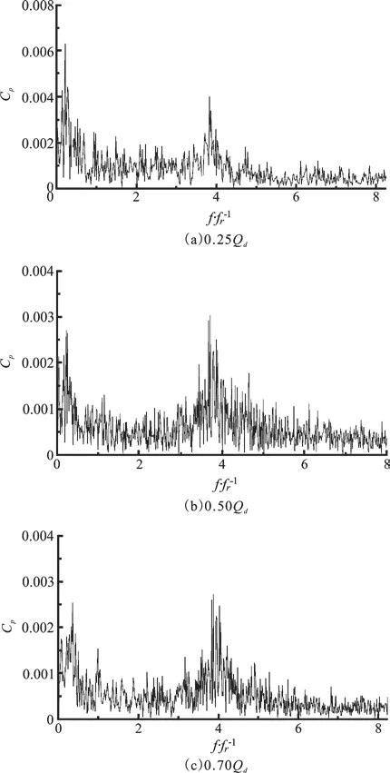
Fig. 6 Frequency spectrum analysis

Figure 5 shows the instantaneous streamline distributions at six equally spaced time steps during one cycle of the main vortex motion obtained by the simulation. The main vortex core starts to move downstream and another small vortex simultaneously appears upstream, to form two counter-rotating vortex pairs with the main vortex. As the small vortex grows larger, the main vortex core is forced to keep moving downstream. Then the main vortex changes dramatically, to be squashed with an increased length. The small vortex is surrounded by exterior streamlines of the main vortex. The two vortexes are emerged together, and a new main vortex is generated. In summary,the main vortex shows its obvious life cycle including decay, split, mergence and growth.

2.2 Stall characteristics

A frequency spectrum analysis is carried out for the series of pressure fluctuations to reveal the stall characteristics. Figure 6 shows the frequency domain of the vibration signals obtained at the location P1 at three different flow rates. It can be seen that the lower frequency is obviously the dominant frequency, which is contributed by the main vortex motion. Further, the“broadband” with a high frequency can also be seen,which is caused by the outlet vortex., the low frequency is 2.6 Hz, only 26.5% of the rotational frequency. While atshown in Figs.6(b), 6(c), the low frequencies are 3.13 Hz, 3.6 Hz,respectively. However, as the flow rate increases, the“broadband” with a high frequency keeps almost the same.

3. Rotating stall

3.1 Flow structures

The rotating stall occurs in the impeller with 5 blades. Figure 7 shows instantaneous streamline distributions at six equally spaced time steps during one cycle of the rotating stall obtained by the simulation.The passage A is taken as an example to analyze the rotating stall. At =0t , we can see the stall cell almost blocks the whole entrance. At 1 6/T, the stall cell becomes larger, and no fluid can flow into the passage A. The fluid is forced to flow into the adjacent passages. In the passage E, the inlet attack angle decreases, and the flow becomes smooth.However, in the passage B, the inlet attack angle increases, then the blade suction surface produces a separation vortex, gradually developing into another stall cell, which eases the block in the passage A.Therefore, the stall cell in the passage A becomes smaller gradually. At 5 6/T, the streamline in the passage A is smooth, but the flow field in the passage B is completely blocked. This mechanism of the rotating stall is consistent with what described in Emmons et al.[20].

3.2 Stall characteristics

In order to determine the propagation speed and direction of the stall cells, the recorded pressure fluctuations on the monitor points P1-P5 are put in the same coordinate frame by transforming the coordinate system, as shown in Fig. 8, where n represents rotor period. At 0. 25Qd, the pressure signals at the points P1-P5 are seen to be fully periodic. The pressure fluctuations on all points have similar periods and amplitudes. But, they have a phase difference, because the stall cells propagate in a circular direction in the impeller. The numbers of stall cells can be calculated as follow

From Fig. 8(a), TCR=3TOSC. Consequently, the number of the stall cells is 3. They propagate from P1-P5 through P2, P3 and P4. In the relative coordinate system, the stall cells rotate in the opposite direction of the impeller rotation. When the flow rate is increased to 0. 5 0 Qd, 0. 60Qd, Figs. 8(b), 8(c) show similar pressure fluctuations observed in Fig. 8(a).According to Eq. (2), the number of stall cells is also 3 at 0. 5 0 Qd, 0. 60Qd. The amplitude of the pressure fluctuations at stall point changes little from 0. 25Qd-0. 60Qd, while the periods during the same time are increased.

A frequency spectrum analysis is carried out for the series of pressure fluctuations to reveal the rotating stall characteristics. Figure 9 shows the frequency domain of the vibration signals obtained at the location P1 at 3 different flow rates. It can be seen that the rotating stall frequency ( fstall) is obviously the dominant frequency, much lower than the rotational frequency. At 0. 2 5 Qd, fstallis 2.4 Hz. While at 0. 5 0 Qd, 0. 6 0Qdshown in Figs. 8(b), 8(c), fstallis 1.73 Hz, 1.4 Hz, respectively.

The propagation speed of the stall cells (ωS) is determined by the angle of the pressure field rotation(Δθ) and the duration of this angle of the pressure field rotation (Δt). Consequently

According to Eq. (3), at 0. 25Qd, the propagation speed of the stall cells is 5.03 rad/s, which is 8% of the rotor speed. While at 0. 5 0 Qd, 0. 60Qdshown in Figs. 9(a), 9(c), it is 3.8% (3.62 rad/s), 1.68% (3.11 rad/s),respectively. Therefore, it can be concluded that the rotating stall frequency is different at different flow rates. With the decrease of the flow rate, the amplitude of the pressure fluctuations tends to be larger, the propagation speed and the rotating stall frequency are lower, but the number remains the same.

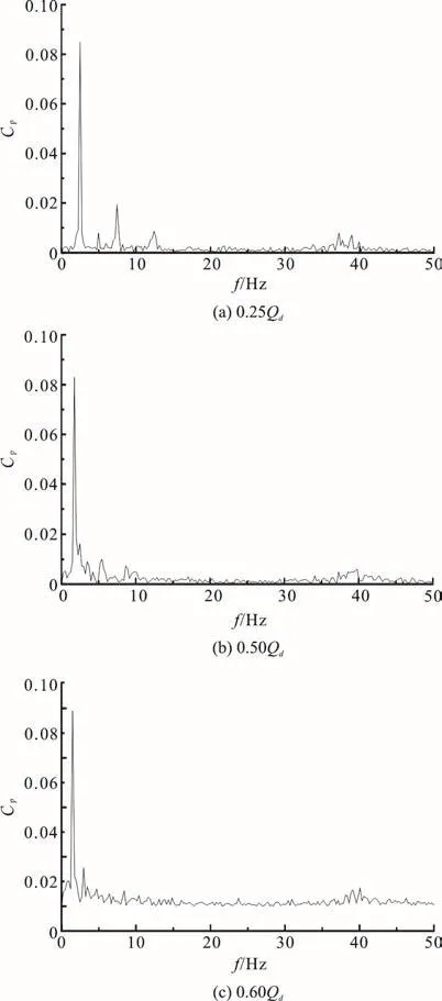
Fig. 9 Pressure fluctuation frequencies

4. Conclusions

The results show that the alternative stall occurs in the impeller with 6 blades, while the rotating stall is observed in that with 5 blades. The conclusions can be obtained as follows:

(1) For the alternative stall, the stall cells are fixed relative to the impeller, but a large vortex in the stalled passage is always swaying. The outlet vortex is generated from it, and then develops and sheds periodically. The pressure fluctuation caused by the outlet vortex motion, acting on the blades, appears as a “broadband” with a high frequency. Further, the large vortex shows an obvious life cycle including decay, split, mergence and growth, which results in a low frequency compared with the impeller passing frequency. With the decrease of the flow rate, the amplitude of the low frequency fluctuation tends to be larger, but the “broadband” with a high frequency keeps almost the same.

(2) For the rotating stall, the stall cells first occur in the suction side of the blade. With the growth of the stall cells, the block area gradually increases until the inlet region is almost blocked, then moves to the pressure side with a continuous decay. When the rotating stall occurs, the amplitude of the pressure fluctuation is much larger than that under the alternative stall condition. The propagation of the stall cells has a significant effect on the pressure fluctuations in the impeller. The dominant frequency of the pressure fluctuation on the blade is the rotating stall frequency. With the decrease of the flow rate, the amplitude of the pressure fluctuations changes little,while the rotating stall frequency decreases.