吴应江,张春明,王攀科,侯 洁

(广东医科大学 生物医学工程学院,广东 东莞 523808)

Alzheimer’s disease (AD) is one of the most common types of neurodegenerative and psychiatric disorders in elderly people worldwide, and the accurate diagnosis of AD, especially for the early stage of the disease, also known as amnestic mild cognitive impairment (MCI), is becoming increasingly important. In the last 20 years, a lot of machine learning models, such as support vector machine (SVM) learning scheme[1], deep learning algorithm[2]and supervised tensor learning (STL) framework which generalize the vector-based learning to the tensor-based learning[3], have been proposed and applied to the classification of Alzheimer disease based on magnetic resonance imaging (MRI) features[4-13].

In the related work, Klöppel applies linear SVM classification to examine different sets of magnetic resonance (MR) images from pathologically proven AD patients and Cognitively Normal (CN) controls[4], while Plant proposes a framework to combine three different classifiers including SVM, voting feature intervals, and Bayes statistics for predicting conversion from MCI to AD[5]. In addition, Abdulkadir assesses the changes in detection performance of a SVM classifier trained with images, which is acquired either with a hardware-only or with different hardwares participated in the Alzheimer’s disease neuroimaging initiative (ADNI) study[6]. It is a large, multi-center and multi-vendor study that acquires structural MRI of AD, MCI and normal healthy controls. Rathore presents a general over-view of pertinent advances in summarizing different AD-related features extracted from neuroimaging data and classification algorithms[7]. Farooq supposes a framework based on convolutional neural network (CNN) for classifying structural MRI images[8]and Sarraf classify AD data from normal control data using CNN deep learning architecture[9], but Bengio noted that supervised deep learning algorithms typically require about 5 000 labeled examples to achieve acceptable performance, and that human-matching performance can be achieved when trained with datasets of more than 10 million labeled examples[2].

Recently, Cuingnet develops a spatial-anatomical regularized SVM framework and successfully applies this framework to the classification of brain MR images[11]. Unfortunately, this framework has two main drawbacks. First, to satisfy the constraints required by traditional single-kernel SVM models, it is necessary to assume that the spatial regularization parameter is equal to the anatomical parameter. However, this assumption is inappropriate because the above-mentioned regularization parameters are not necessarily the optimal values and the solution of this kind of optimization problem is very complicated and time-consuming. Although Cuingnet points out two parameters could have differed, it is more difficult to tune the parameters because of high computational complexity and it is also difficult to merge the two regularization terms into one term in a single kernel model. Secondly, in SVM optimization scheme, it needs to reshape a 3D MRI brain image naturally represented by a multi-dimensional array to a one-dimensional vector so that the vectorial input requirement is met. In this way, when constructing the spatial kernel function in the framework, it is inevitable to use a large-scale matrix to express the adjacency relationship between each pair of vertices, resulting in high time and space complexity.

In this paper, in order to overcome the first drawback of Cuingnet framework, we propose an approach to improve the framework by combining Multiple Kernel Learning (MKL)[14-15]with the widespread Sequential Minimal Optimization (SMO) algorithm[16]to solve the optimization problem of parameter estimation for spatial and anatomical regularizations. In order to overcome the second drawback of Cuingnet framework, we design small-scale matrices derived from every slice of MRI neuroimaging data to retain spatial and anatomical adjacencies in the construction of multislice kernel. The present paper extends our previously published work[17-18], develops the basic theory of the precondition of kernel functions manipulation, provides an in-depth analysis on how to effectively combine kernel functions respectively associated with spatial and anatomical structure information in a MRI image, and how to reduce the complexity involving in spatial kernel function computation. To demonstrate the performance of the proposed new approaches, all the MRI images in [10,19] and [17-18,20] are selected and compared with classification of probable AD versus normal controls, and the results indicate that the new methods outperform previous ones in computational complexity while high classification accuracy is maintained.

1 Materials and methods

1.1 Preliminaries on kernel-based learning In this section, some traditional notation is introduced firstly, and then the precondition of manipulation of different kernel functions are discussed. Scalars are represented in italic lowercase letters, e.g.,a; vectors are represented in boldface italic lowercase letters, e.g.,a; matrices are represented in italic capitals letters, e.g.,A; tensors are represented in boldface italic capitals letters, e.g.,Aand spaces are represented in capitals letters, e.g., A.

In traditional kernel-based learning, it is assumed that Ω is a nonempty set and a kernelkis a real-valued function defined on Ω×Ω,kis symmetric if, for anyx,y∈Ω, it satisfiesk(x,y) =k(y,x), andkis positive definite if, for anyN≥1 and anyx1,x2,...,xN∈Ω, it satisfies Σijcicjk(xi,xj) ≥ 0 for allc1,c2,...,cN∈R. Hence,kis a positive kernel on Ω×Ω ifkis symmetric and positive definite. It is notable that postitive definite kernels are also called reproducing kernels or kernels[21].

The class of kernels on Ω×Ω has beautiful closure properties. In particular, it has been demonstrated that this class is closed under addition, multiplication by a positive constant and direct product, that is, ifk1(x,y) andk2(x,y) are kernels, thenk1(x,y)+k2(x,y),ck1(x,y) andk1(x,y)k2(x,y) are kernels wherec∈R+[22]. Therefore, a linear combination with positive coefficients of kernel functions defined on the same space is still a kernel function. Furthermore, a precondition of manipulation of different kernel functions is that all the kernels are defined on the same space, and one only has to ensure that the kernels are positive definite which in turn guarantees the kernel manipulated on the same space is a valid reproducing kernel.

Haussler proves that if Ω is a separable metric space andkis a continuous kernel, there exists only a reproducing kernel Hilbert space associated with kernelk[23]. Furthermore, Haussler proposes an approach to build kernels on sets whose elements are discrete structures such as strings, trees and graphs, and puts forward the concept of convolution kernel and provides a method to construct a kernel on an infinite set from kernels involving generators of the set.

In addition, Haussler proposes the concept of convolution kernel, suggests a method to construct a kernel on a set whose elements are discrete structures (such as strings, trees and graphs), and provides an approach to build a kernel on an infinite set from of set generating kernels.

Kondor constructs a natural class of kernels on graphs[24]based on spectral graph theory. First, the exponential of a square matrixHis defined as formula (1)：

(1)

This limit always exists and formula (1) may be derived using Taylor’s expansion as formula (2)：

(2)

IfHis symmetric, it could be verified that the exponential ofHis symmetric and positive semi-definite. In other words, this exponential matrix is a candidate for a kernel.

Therefore, an exponential family of kernels may be constructed as formula (3)：

k=eβH

(3)

whereHis generator and β is bandwidth parameter.

The above kernels are called diffusion kernels or heat kernels because the resulting differential equation is analogous to classical physics equations which are used to describe the diffusion of heat. Finally, Kondor design a generator as formula (4)：

(4)

wherei～jdenotes verticesviandvjthat connected by an edge,diis the degree of vertexvi, and the negative of matrixHis defined as the Laplacian matrix of the graph.

1.2 Cuingnet framework SVM is currently considered as one of the most effective learning method, which is based on statistical learning theory proposed by Vapnik in the 1990s[1]. Let input training dataset as T={(xs,ys),s∈1, 2, …,N} wherexs∈Ω,ys∈{+1, -1} and Ω is the input space, then the primal optimization problem of SVM may be formulated as formula (5)：

(5)

where λ∈R+is a regularization parameter that controls the trade-off between the two terms, andlhingeis the hinge loss function.

LetLdenote the Laplacian matrix associated to a connected graph and the size of regularization is regulated by parameter β, the primal SVM solution can be reformulated as formula (6)：

(6)

Voxels of a 3D MRI brain image can be considered as nodes of a graph, and the image connectivity (e.g., 6-connectivity) is one of the simplest ways to encode spatial structure information. LetLsdenote the Laplacian matrix of a graph encoding spatial structure information and it is also called spatial Laplacian matrix for brevity. By means of a symmetric orthogonal matrixQ, the imaginary part of discrete sine transform (DST) matrix,Lscan be converted to a diagonal matrixS. In other words, the matricesQandSmay be formulated respectively as formula (7) and (8)

0≤m,n≤d-1

(7)

S=Q*Ls*Q

(8)

whereLs,Q,Sared×ddimension matrices,d=I1*I2*I3, and the MRI image size isI1×I2×I3. Furthermore, the spatial exponential matrix may be calculated as formula (9)：

e-βsLs=e-βsQSQ=Qe-βsSQ

(9)

Finally, the computational complexity of the exponential matrix is O [(I1*I2*I3)6].

Similarly, the probability that two voxels belong to the same anatomical region is the most effective means of encoding anatomical structure information. LetLadenote the Laplacian matrix of a graph encoding anatomical adjacency relation and it is also called anatomical Laplacian matrix for brevity. In this manner, the anatomical exponential matrix may be calculated and the detailed calculation procedures are described in [17] [19].

In order to introduce spatial and anatomical structure information into SVM model, two regularization terms are combined to yield the following optimization problem in formula (10)：

(10)

where λsdenotes the spatial regularization parameter and λadenotes the anatomical regularization parameter, βsand βaare corresponding diffusion parameters.

Unfortunately, this framework has two main drawbacks. First, for the purpose of satisfying the restrictive conditions required in classical single kernel SVM model, it makes an assumption that the spatial regularization parameter is equal to the anatomical one, that is,λs=λa=λ, so as to the spatial and anatomical regularization terms could be integrated into one term. However, this assumption is improper because λs=λa=λ is not necessarily the optimal values and the computation of gram matrix via the equations in [19] is very complicated and has very high computational complexity. Although Cuingnet points out that the regularization parameter λsand λacould have differed, it is more difficult to tune up the two weight parameter values because run-time complexity is very high. Furthermore, in a single kernel model, it is not feasible to merge the two regularization terms into one term when the values of two regularization parameters are not equal. Second, in order to meet the input conditions of the classic SVM model, it is necessary to convert 3D MRI brain images, which are generally represented by high-order tensors in nature, into one-dimensional vectors. However, this transformation destroys the inherent structure and the correlation of an original image, and generates high-dimensional vectors. In this manner, a conventional voxel connectivity structure, such as the 6, 18, or 26-neighborhood, should be employed to define the neighbors of each voxel. Therefore, a large-scale spatial adjacency matrix is unavoidably used to define the adjacency relation between every pair of vertices during the construction of spatial kernel function in this framework and thus it will produce a very high time and space complexity.

1.3 Tensorial kernel function with spatial and anatomical structure information

1.3.1 Parameter optimization based on MKL method In order to overcome the first drawback of Cuingnet framework, we propose a method to solve this parameter optimization problem based on Kloft method [14] and SMO-MKL algorithm[15].

Kloft devises two efficient interleaved optimization strategies by imposing ap-norm penalty on the kernel combination coefficient, and this interleaved optimization is much faster than the commonly used wrapper approaches[14]. There is an important hypothesis for Kloft method that it is givenMdifferent feature mappingsψm：X→Hm,m=1, 2, …,M, e and each one gives rise to a reproducing kernelkmof Hm. That is to say, all the kernels should be defined on the same space with satisfying the precondition of manipulation of different kernel functions. Therefore, convex approaches to multiple kernel learning may consider ask=Σdmkm,dm≥0, namely, a nonnegative linear combination of base kernel functions which defined on the same space.

(11)

(12)

In view of the problems studied in this paper,it is quite easy to see that the regularization parameter λsand λacorresponding tod1andd2, respectively.

Finally, SMO-MKL algorithm is developed for optimizing thelp-MKL formulation and the optimal regularization parameters, λsand λa, may be computed according to formula (12) by means of the above two kernel functions. The kernel matrix-related code in LIBSVM[25]and SMO-MKL should be rebuilt so as to search the optimal values of various parameters and calculate these pre-computed kernel matrices.

1.3.2 Multislice kernel function In order to overcome the two drawbacks of Cuingnet framework mentioned above, we construct two new multislice kernels in this section, wherein small-scale adjacency matrices derived from every slice of a 3D MRI brain image are adopted to retain spatial and anatomical adjacencies, so that the large amount of computation is circumvented while high classification accuracy is maintained. At the same time, the SMO-MKL algorithm is also adopted to determine the optimal regularization parameters.

As you can see from Fig.1, the adjacency matrix of every frontal slice of a 3D MRI brain image will retain the adjacency relation of vertices in the XY plane. Analogously, adjacency matrices of lateral and horizontal slices will respectively retain the adjacency relation of vertices in the YZ plane and XZ plane. Therefore, if we combine these three kinds of adjacency matrices, we will effectively build the adjacency relation between every pair of vertices.

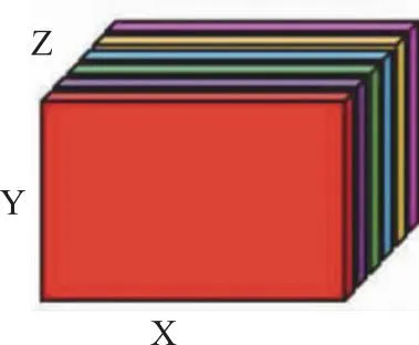
Fig.1 Frontal slices

Let input training dataset as T={(Xi,yi),i∈1, 2, …,M}, whereXi∈RI1×I2×…×IN,yi∈{-1,1} andNis the order of the tensor. We may transform the input space into a higher-dimensional tensor product feature space using a mapping functionφ：X→φ(X)∈RH1×H2×…×HP, and then the optimization problem of SVM classifier in the tensor setting may be formulated as formula (13)[3]：

s.t.yi(+b)≥1-ξi

ξi≥0,∀i=1,…,m

(13)

whereW∈RH1×H2×…×HPdenotes a weight tensor.

Once the above model is solved, the class label of a testing exampleXcan be predicted as formula (14)[3]：

(14)

In formula (14), it is crucial to predefine the tensorial kernelk(Xi,X) and calculate the set of parameters ψiwithi=1, 2, …,m. Among them, the first step is the more critical.

Recently, Signoretto presents a kernel-based framework to the tensorial data analysis[26]. The major contribution of this framework is that it defines the tensorial kernel function ask(X,Y)=k1(X,Y)k2(X,Y)…kN(X,Y), whereX(i)is the mode-imatricization of tensorX, andY(i)is the mode-imatricization of tensorY. The kernelki(X,Y) is constructed from matrixX(i)andY(i),i=1, 2, …,N,XandYmust have the same sizeN. The Signoretto framework is more effective whenki(X,Y) is designed to be a Gaussian-RBF kernel function since Gaussian-RBF kernel function is an exponential function, and if we take the product of two exponential expressions with the same base, we simply add the exponents. However, this simple and convenient calculation will be lost whenki(X,Y) is designed to be a heat kernel function or other kernel function. In addition, since the mode-imatricization will be carried out in the beginning of the algorithm, if we try to include the spatial structure information of an MRI neuroimaging datum, this procedure will also lead to a huge dimensional adjacent matrix and generate the high computation complexity. To circumvent this problem, we propose to design tensorial kernel function simultaneously including spatial and anatomical structure information, and solve the associated SVM modeling problems with the designed kernel functions.

The first tensorial kernel function constructed in our study is named Zero-Extended-Kernel. It is worth mentioning that all tensorial kernel functions should be defined on the same space to satisfy the precondition of SMO-MKL model. LetImax=max{I1,I2,I3}, and a 3D MRI brain image can be extended fromRI1×I2×I3toRImax×Imax×Imaxby defining gray valuef(x,y,z) = 0. If voxel (x,y,z) is not inRI1×I2×I3, then this zero-extension scheme can be formulated as formula (15)：

(15)

Hence, all horizontal, lateral and frontal slices of MRI images have the same sizeImax×Imax. It is easy to know that all the spatial and anatomical Laplacian matrices and all the exponential matrices generated from these Laplacian matrices are equal in size. Consequently, all the kernel functions are built up from these slices and belong to the same spaceRdmax×dmaxwheredmax=Imax*Imax, and thus meet the precondition of the SMO-MKL method. It should be pointed out that the above kernel functions will not increase the computational burden because all gray values in the extension equal to zeros so they are not used in the actual computation of kernel functions.

With the definition of the third-order tensor inner product, a linear kernel function is constructed as formula (16)[27]：

klinear(X,Y)=

(16)

Formula (16) indicates that vectorization is the essence of the inner product of two same-sized tensors, and, consequently, the linear kernel function of the two 3rd-order tensors is the sum of the products derived from vectorizing the corresponding frontal slices of tensorsXandY. Since the structural information within the slice is lost with vectorization, a kernel function generated from Laplacian matrix is provided to alleviate the problem.

Therefore, a new kernel function of the third-order tensor is generated as formula (17)：

(17)

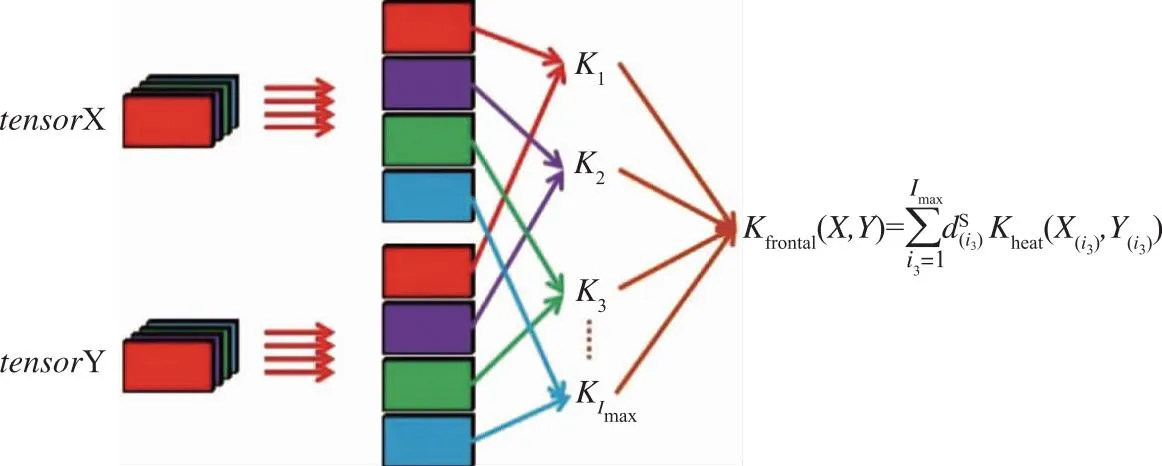
Fig.2 Third-order tensor kernel function

Similar procedures can be repeated on the horizontal and lateral slices of a 3rd-tensor respectively, and thus a tensorial kernel function including spatial structural information may be formulated as：

kspatial(X,Y)

= khorizontal(X,Y) + klateral(X,Y) + kfrontal(X,Y)

(18)

The above idea can be easily extended to construct kernel functions with anatomical regularization. Therefore, a new tensorial kernel function containing both spatial and anatomical structure information is formulated as formula (19)：

kZero - Extended - Kernel(X,Y)

(19)

With the above kernel function in formula (14), then SVM learning scheme in the tensor setting is converted to an MKL problem and thus it can be solved efficiently using the SMO algorithm. In this way, the computational cost of this tensorial kernel matrix is decreased from O [(I1×I2×I3)8] to O [(I1×I2)8×I3+(I2×I3)8×I1+(I1×I3)8×I2]. Furthermore, it’s obvious that Spatial-Tensor-Kernel in [15] is a special case of Zero-Extended-Kernel.

We may construct another tensorial kernel named Frontal-Horizontal-Kernel. In fact, the size of a pre-processed image isI1×I2×I3=121×145×121, hence the sizes of horizontal slice, lateral slice and frontal slice areI2×I3=145×121,I1×I3=121×121,I1×I2=121×145, respectively. That is to say, horizontal slice and frontal slice have the same size. Therefore, the corresponding spatial and anatomical Laplacian matrices and exponential matrices generated from these Laplacian matrices also have the same size. Consequently, all the kernel functions derived from these slices belong to the same spaceRd*×d*whered*=121*145, and meet the prerequisites for the SMO-MKL method.

Finally, following a similar procedure as described above, another new tensorial kernel function including the spatial and anatomical structure information is obtained as formula (20)：

kFrontal - Horizontal - Kernel(X,Y)

(20)

Similarly, the computational cost of this tensorial kernel matrix is decreased from O ((I1×I2×I3)8) to O [(I1×I2)8×I3].

2 Experimental results

The 3D MRI brain images used in this study are from the same population that mentioned in the first part. In these studies, 299 subjects are selected from the ADNI dataset (http：//adni.loni.usc.edu), including 162 CN controls and 137 patients with AD.

By using the Statistical Parametric Mapping (SPM) and Voxel-Based Morphometry (VBM) toolbox, gray matter (GM), white matter (WM) and Cerebrospinal Fluid (CSF) features with the default parameters are computed, and by using the Diffeomorphic Anatomical Registration through Exponentiated Lie Algebra (DARTEL) tools more accurate inter-subject registration of brain images are achieved. A major change from SPM5 to SPM8 is that the latter implements a number of new routines which provide for a robust and efficient source reconstruction using Bayesian approaches. Therefore, contrasting approaches to the Cuingnet study, the critical pre-processing steps of the proposed method are the structural brain image segmentation with SPM8 package, the generation of GM/WM/CSF average template and optimized deformation field with DARTEL algorithm, and the normalization of the segmented image to Montreal Neurological Institute (MNI) Space. It is worthwhile to note that the overall tissue amount should remain unchanged during modulation of all GM/WM/CSF densities in the MNI standard space. Fig.3, Fig.4 and Fig.5 are the results of the three pre-processing steps for a 3D MRI brain image, respectively.

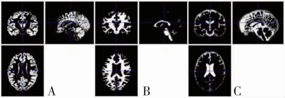
A： GM. B：WM. C： CSF.Fig.3 Structural brain image segmentation

In this experiment, a grid search method and 10-fold cross-validation strategy are adopted to obtain optimal parameter values. As combining spatial and anatomical regularization with the same parameter β in Cuingnet framework, we also assume that diffusion parameter βs=βa=β. Furthermore, according to our experiment, we need to search for diffusion parameter in β=1.25, 1.5, 1.75, 2, 4 and 6 respectively because the optimal parameter value is quite close to the value 1.75. Table 1 presents the results of a randomized experimental evaluation of Spatial-Anatomical-MKL method with different β. It should be noted that a single anatomical regularization kernel has a rapid decline in accuracy (Acc.) when diffusion parameter β>2, while a single spatial regularization kernel with the same parameter value has a high accuracy rate. Therefore, by combining MKL with the widespread SMO method, integrating spatial and anatomical regularization still achieves high accuracy if spatial regularization kernel is given a greater weightw2. Given the classication accuracy does not enable to compare the performances between the different classication experiments, sensitivity (Sens.) and specificity (Spec.) is also considered. All algorithms are conducted in MATLAB (R2010a) on Windows XP running on a Lenovo ThinkStation with system configuration Intel(R) 3.4 GHz CPU with 32 GB of RAM.

The results of the classification experiments for Cuingnet framework VS Spatial-Anatomical-MKL are summarized in Table 2. The lowest accuracy is obtained with Voxel-Regual-Combinegraph and the highest with Spatial-Anatomical-MKL. From the above results we know that it is unreasonable to assume λs=λaand they are not the optimal parameters values.

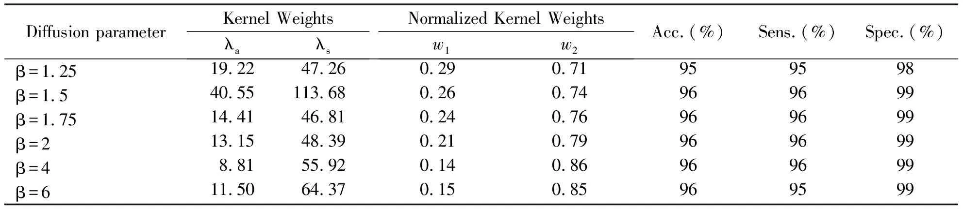
Tab.1 Classification performances of Spatial-Anatomical-MKL method with different parameter

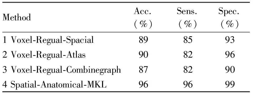
Tab.2 Performance comparison of Cuingnet and Spatial-Anatomical-MKL method

As shown in Table 5, Voxel-Regual-Combinegraph, Spatial-Anatomical-MKL, Spatial-Prior-in-STM and Spatial-Tensor-Kernel algorithm yield peak accuracies of 89%, 96%, 93% and 95%, respectively. In comparison, it can be observed that the proposed Zero-Extended-Kernel reach peak accuracies of 97% and Frontal-Horizontal-Kernel algorithms with 96%. Therefore, Zero-Extended-Kernel yields the highest classification accuracy due to the construction of the tensorial kernel function and the two problems of Cuingnet framework are solved effectively.

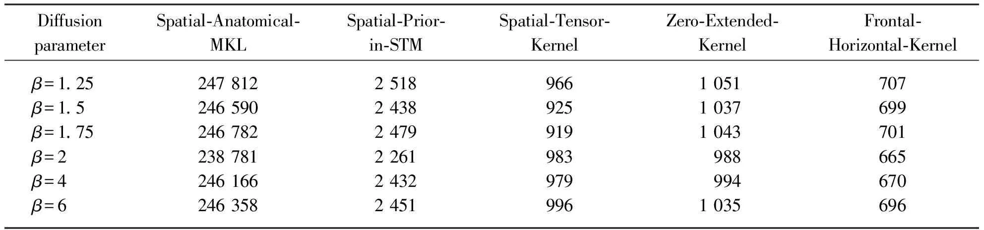
Tab.3 Running time (seconds) of proposed method with different parameter

Tab.4 Classification performances of proposed method with different parameter

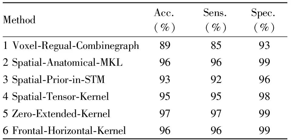
Tab.5 Performance comparison of different methods

3 Conclusion

Magnetic resonance imaging (MRI) image analysis is one of the most active research areas in image processing theory and application. It is also an important method for clinical diagnosis for patients with AD. Aiming at existing problems in current AD-related MRI image classification[4-13], in this thesis, we focus on algorithms for automatic classification of AD-related MRI images based on vector multi-kernel learning and tensor multi-kernel learning. At the same time, based on the basic theory and the precondition of kernel function operation in the same space[1-3], this thesis provides an in-depth analysis on how to effectively combine kernel functions respectively associated with spatial and anatomical structure information in a MRI image, and how to reduce the complexity involving in spatial kernel function computation. The kernel functions containing spatial and anatomical information based on the above theory are applied to the classification of AD-related MRI image data. The main contents and innovations are as follows： (1)AD Brain MRI Image Classification Based on Vector Multi-kernel Learning;(2) AD Brain MRI Image Classification Based on Tensor single-kernel Learning;(3) AD Brain MRI Image Classification Suspected Based on Tensor Multi-kernel Learning.

Firstly, the existing classification algorithm of AD-related MRI data based on traditional vector single-kernel learning is studied and the advantages and disadvantages of the classical Cuingnet framework are also analyzed. In the related work, Cuingnet proposed a general classification framework to introduce spatial and anatomical structure information in classical single-kernel support vector machine (SVM) optimization scheme for brain image analysis, which has achieved good classification accuracy. However, this framework has two main drawbacks. First, it involves spatial and anatomical regularization and in order to satisfy the optimization conditions required in the single kernel case, it is pre-assumed that the spatial regularization parameter value is equal to the anatomical one. Second, in the framework it has to convert a 3D discrete brain image, which is generally and naturally represented by a higher-order tensor, to a one-dimensional vector in order to meet the input requirements. In this manner, the natural structure in the original data is destroyed, and what is worth, generally it produces a very high-dimensional vector so that the famous problem of curse-of dimensionality in machine learning will become more serious, and at the same time, a huge adjacency matrix is unavoidably adopted during the construction of spatial kernel, to determine the adjacency relation between each pair of voxels, which leads to very high time and spatial complexity.

To overcome the first drawback in the Cuignet framework, i.e., spatial and anatomical regularization parameters are pre-assumed to be equal, in this thesis we propose an improved method named Spatial-Anatomical-MKL (multiple kernel kearning) to combine the sequential minimal optimization (SMO) algorithm with MKL to solve the optimization problem of regularization parameter estimation. We first prove that the spatial and anatomical kernel functions in the Cuingnet framework can satisfy the preconditions of the Kloft model and the SMO-MKL algorithm, so that the spatial and anatomical kernel functions can be linearly combined and the weight coefficients of these kernel functions can be properly determined. Therefore, the Spatial-Anatomical-MKL method effectively solves the first problem in the Cuingnet framework and it also extends the algorithm for classification of AD-related MRI data from vector single-kernel learning to vector multi-kernel learning. However, the second problem in the Cuingnet framework, that is, a huge adjacency matrix is unavoidably adopted to determine the adjacency relation between each pair of voxels, still remains unsolved in the Spatial-Anatomical-MKL method and thus the computational complexity is still high.

To overcome the second drawback of high computational complexity in spatial kernel calculation in the Cuignet framework, this thesis proposes an improved method named Spatial-Prior-in-STM based on support tensor machine (STM). First, we perform a more detailed analysis of alternating iterative algorithm of classical rank-1 STM and then proposed an improved version wherein the iterative process is divided into two steps so that the canonical decomposition / parallel factors (CP decomposition) and spatial structure information of all frontal slices of an MRI image is included in the classic rank-1 STM model, in a manner that many smaller adjacency matrices of frontal slices are adopted to retain the spatial structure information and to reduce the space and time overhead. However, due to the limitation of the alternating iterative algorithm, the Spatial-Prior-in-STM method only contains the spatial structure information of all frontal slices of MRI data and cannot include the spatial structure information of any horizontal and lateral slices and the anatomical structures information of all kind of slices of MRI data simultaneously.

Therefore, two novel tensorial kernels based on the spatial and anatomical structure information are proposed for AD classification in this paper. To preserve the spatial and anatomical adjacency relation, the spatial and anatomical Laplacian matrices derived from each slice are incorporated into the construction of these tensorial kernels. The experiment results show that the proposed two new methods outperform previous ones in computational speed while maintaining high classification accuracy. In our study, we employ the classical inner product of two same-sized tensors, determined by the sum of product of the corresponding elements, thus potentially breaking the intrinsic structure of tensor data. Therefore, part of our future work is to find new definitions of tensor inner products so that the intrinsic structural information contained in tensors is preserved.