ZuHan Liu , JianHua Xu , WeiHong Li

1. Jiangxi Provincial Key Laboratory of Water Information Cooperative Sensing and Intelligent Processing, Nanchang Institute of Technology, Nanchang, Jiangxi 330099, China

2. Key Laboratory of Geographic Information Science (Ministry of Education), School of Geographic Sciences, East China Normal University, Shanghai 200241, China

3. Research Center for East-West Cooperation in China, East China Normal University, Shanghai 200241, China

4. State Key Laboratory of Desert and Oasis Ecology, Xinjiang Institute of Ecology and Geography, Chinese Academy of Sciences, Urumqi, Xinjiang 830011, China

Complex network analysis of climate change in the Tarim River Basin, Northwest China

ZuHan Liu1,3, JianHua Xu2,3*, WeiHong Li4

1. Jiangxi Provincial Key Laboratory of Water Information Cooperative Sensing and Intelligent Processing, Nanchang Institute of Technology, Nanchang, Jiangxi 330099, China

2. Key Laboratory of Geographic Information Science (Ministry of Education), School of Geographic Sciences, East China Normal University, Shanghai 200241, China

3. Research Center for East-West Cooperation in China, East China Normal University, Shanghai 200241, China

4. State Key Laboratory of Desert and Oasis Ecology, Xinjiang Institute of Ecology and Geography, Chinese Academy of Sciences, Urumqi, Xinjiang 830011, China

The complex network theory provides an approach for understanding the complexity of climate change from a new perspective. In this study, we used the coarse graining process to convert the data series of daily mean temperature and daily precipitation from 1961 to 2011 into symbol sequences consisting of five characteristic symbols (i.e., R, r, e, d and D), and created the temperature fluctuation network (TFN) and precipitation fluctuation network (PFN) to discover the complex network characteristics of climate change in the Tarim River Basin of Northwest China. The results show that TFN and PEN both present characteristics of scale-free network and small-world network with short average path length and high clustering coefficient. The nodes with high degree in TFN are RRR, dRR and ReR while the nodes with high degree in PFN are rre, rrr, eee and err, which indicates that climate change modes represented by these nodes have large probability of occurrence. Symbol R and r are mostly included in the important nodes of TFN and PFN, which indicate that the fluctuating variation in temperature and precipitation in the Tarim River Basin mainly are rising over the past 50 years. The nodes RRR, DDD, ReR, RRd, DDd and Ree are the hub nodes in TFN, which undertake 19.71% betweenness centrality of the network. The nodes rre, rrr, eee and err are the hub nodes in PFN, which undertake 13.64% betweenness centrality of the network.

climate change; complex networks; coarse graining process; temperature fluctuation network; precipitation fluctuation network; Northwest China

1 Introduction

Climate change and its effects on human society are matters of widespread concern and have received increased attention from the public worldwide, and temperature and precipitation are the two important climate factors affecting human economies and terrestrial ecosystems.

A number of studies (Palmer, 1999, 2000; Liston and Pielke, 2000; Rial et al., 2004; Martínez et al.,2007; Livada et al., 2008; Brunsell, 2010; Fan et al.,2011, 2013; Li et al., 2011a,b, 2013; Xu et al.,2011a,b, 2016a; Du et al., 2013; Liu et al., 2013,2017) indicate that climate is a complex system where temporal and spatial variations have been taking place at a global, regional and local scale over the past few centuries. Therefore, it is necessary to further understand the mechanisms of climate change from a variety of perspectives (Xu et al., 2010).

However, climate has been identified as a set of atmospheric states of a dynamic, chaotic system showing deterministic variability (Lorenz, 1991). The interpretation of climate as a complex intervariable organization is a key issue for understanding climatic processes (Millán et al., 2009; Nie et al., 2012; Liu et al., 2014a,b). Although some articles (Fraedrich,1986; Tsonis and Elsner, 1988; Rodriguez-Iturbe et al., 1989; Zeng et al., 1992) discussed and explained the nonlinear variation of climatic parameters such as precipitation, temperature, relative sunshine duration,and wind velocity, the extension of these studies is still limited due to the complexity of climatic systems(Xu et al., 2013a,b,c, 2014a). Facing climate change with frequent extreme weather events (Katz and Brown, 1992), understanding the complexity of climate system is still a difficult problem, which requires further in-depth investigation (Xu et al., 2011,2016b).

The complex network theory developed over the last decade provides an approach for understanding the structure, stability, statistical law and dynamic mechanism of networks. In particular, the small-world networks (Watts and Strogatz, 1998) and scale-free networks (Barabási and Albert, 1999) reveals the basic features of a large number of complex networks.This theory has been widely used in nature and human society. That is because many complex systems can be abstracted as a network composed of interactional individual (Albert and Barabási, 2002), for instance, the Internet (Faloutsos et al., 1999; Vázquez et al., 2002; Barrát et al., 2005), World Wide Web(Barabási and Albert, 1999; Adamic et al., 2000; Albert et al., 2000), air pollution (Sun et al., 2016), temperature (Zhou et al., 2008), railway (Hossain and Alam, 2017), social (Lymperopoulos and Ioannou,2016; Rezvanian and Meybodi, 2016), airline (Barrát et al., 2005), ecological (Montoya et al., 2006), company relationships' (An et al., 2016), protein-protein interaction (Maslov and Sneppen, 2002), power(Watts and Strogatz, 1998; Liljeros et al., 2001), economic (Rendón et al., 2016) and scientific collaboration networks (Barrát et al., 2005). The analysis method of complex networks provides a tool to understand the structural properties of climate change from a new perspective (Steinhaeuser et al., 2011; Feldhoff et al.,2015), and climate networks have emerged as a strong analytical framework for both descriptive analysis and predictive modeling of the emergent phenomena. For example, complex networks can effectively discover climatic indices (Saha and Mitra, 2015), reduce the uncertainty of climate extremes (Steinhaeuser et al.,2009), discriminate different types of El Nino or La Nina events (Wiedermann et al., 2016) and distinguish the effects of internal and force atmospheric variability (Deza et al., 2014). To further understand the complexity of climate change in the Tarim River Basin, Northwest China, based on daily data at 23 meteorological stations during the period from 1961 to 2011, this study constructed the temperature fluctuation network (TFN) and precipitation fluctuation network (PFN) using the coarse graining process (Zhou et al., 2008) and investigated the complexity of temperature and precipitation processes.

2 Study area and data

The study area is the Tarim River Basin, located between longitudes 73°10′E~94°05′E and latitudes 34°55′N~43°08′N, which covers an area of 1.02X106km2(Chen et al., 2006). This area has a typical desert climate with an average annual temperature of 10.6~11.5 °C, monthly mean temperature ranges from 20 °C to 30 °C in July and −10 °C to −20 °C in January. The highest and lowest temperatures are 43.6 °C and −27.5 °C, respectively. The accumulative temperature >10 °C ranges from 4,100 °C to 4,300 °C.Average annual precipitation is 116.8 mm in the basin, and ranges from 200 mm to 500 mm in the mountainous area, 50 mm to 80 mm in the edges of the basin and only 17.4 mm to 25.0 mm in the central area of the basin. There is great unevenness in the precipitation distribution within any year. More than 80% of the total annual precipitation falls between May and September in the high-flow season, and less than 20% of the total falls from November to next April (Xu et al., 2009, 2014b).

To study the complexity of climate change in the Tarim River Basin, we used daily average temperature and daily precipitation data from 23 meteorological stations (Figure 1) spanning from 1961 to 2011 in the Tarim River Basin. This data is from the Information Center of Meteorological Office in Xinjiang Uygur Autonomous Region, so the accuracy and exact error can be ensured.

3 Theory and methods

Our analysis builds on the theory and methods of complex networks as follows.

3.1 Complex network

The last decade has witnessed the study of complex networks, i.e., networks whose structure is irreg-ular, complex and dynamically evolving over time,with the main focus moving from the analysis of small networks to that of systems with thousands or millions of nodes, and with a renewed attention to the properties of dynamical units' networks (Boccaletti et al., 2006). The complex networks with non-trivial topological features do not occur in simple networks such as lattices or random graphs but often occur in graph modelling of real systems.

The characteristics of a complex network are mainly as follows: (a) the number of nodes are huge diverse, which can represent anything (e.g., the nodes represent individuals in the network of interpersonal relationships, while representing different homepages in the climate networks); (b) multiplex connections(edges) possibly with directionality and the connection (edge) weights between nodes are different; (c)nodes and connections between nodes maybe generate or lost at any time, which result in a constantly changing network structure; and (d) its dynamic is a complex non-linear system.

Compared with traditional networks in the graph theory (Newman, 2010), the significance of complex networks are as follows:

(1) All the traditional networks are small networks, and the numbers of nodes often are dozens to hundreds, whereas the number of nodes in a complex network often are many thousands, even as many as a million. The large number of nodes greatly increases the complexity of the network.

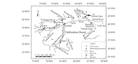
Figure 1 Locations of meteorological stations in the Tarim River Basin

(2) The complex network theory provides us with a new insight, enabling us to explore the law or characteristics of complex networks hiding in a huge number of nodes and their connections. Its significance is beyond the traditional network.

(3) Traditional network analysis mainly relies on mathematical reasoning and mapping techniques.However, for complex networks, computing and mapping tasks are processed by computers.

(4) Compared with traditional networks, complex networks cover a wide range of topics, across natural and social sciences and other fields, such as physical,sociological and biological research areas.

3.2 Characterization of complex networks

Complex networks are often characterized by indicators such as degree, degree distribution, average path length, clustering coefficient, and betweenness centrality.

(1) Degree and degree distribution

According to the definition in graph theory, the degree of a node in a network is the number of connections (edges) it has to other nodes. If eijrepresents a connection (edge) from node i to node j, the degree of the node i can be calculated as

where V represents the set that includes all nodes in the network.

If the studied network is a directed network, then node i has two degrees, namely, out-degree and in-degree. The out-degree is calculated as

The in-degree is calculated as

The total degree of node i is as follows:

The average degree of the network is defined as

where < k > represents the average degree of the network, and N is the total number of nodes in the network.

Degree distribution is the probability distribution of different degrees in the network (Newman, 2001).The degree distribution P(k) of a network is usually defined to be the proportion of nodes with degree k to the total number of nodes in the network. Obviously,P(k) is also the probability of the selected nodes whose degree equal k under the principle of stochastic consistency. A histogram can be used to represent the degree distribution of a network.

Based on the degree distribution of a network, we can further define the cumulative degree distribution of the network as

Figure 2 shows two kinds of degree distribution of the networks, i.e., (a) Poisson distribution and (b)power-law distribution. The Poisson distribution is a hill-shaped distribution in which the average degree of the network has the greatest probability of occurrence and the probability of the node appearing becomes smaller with the deviation from the average degree increases. The power law distribution shows a linear distribution of the fat tail, in which the number of nodes decreases with increasing degree.

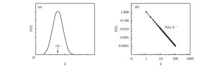
Figure 2 (a) Poisson distribution and (b) power-law distribution

(2) Distance and average path length

In a network, the distance (path length) between two nodes is defined as the length of the shortest path between two nodes. The diameter of a network is defined as the maximum distance between any two nodes in the network. The average path length of the network is defined as the average of the distance between all pairs of nodes, which describes the degree of separation between the nodes in the network.

The average path length of the network is calculated as

where L represents the average path length of the network; dijis the shortest path length from node i to node j; and N is the total number of nodes.

Formula (7) contains the distance from each node to itself, and eliminates the problem of isolated points in the network.

(3) Clustering coefficient

The clustering coefficient is a measure of the number of triangles in a network. The clustering coefficient of a network is based on a local clustering coefficient for each node.

The clustering coefficient of node i is defined as

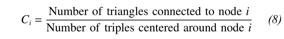
where a triple centered around node i is a set of two edges connected to node i. If the degree of node i is 0 or 1, which gives us Ci=0/0, we can set Ci=0.

The clustering coefficient for the whole network is the average of the local values Ci, i.e.,

where N is the number of nodes in the network. It is evident that we have 0≤Ci≤1 and 0≤C≤1.

The clustering coefficient of a network is closely related to the transitivity of the network, which measures the relative frequency of triangles.

For the weighted network (edge-weighted), the clustering coefficient of node i is defined as

where wijdenotes the weight of the edge connecting nodes i and j; kiis the degree of node i; aijis the element of adjacency matrix, which equals 1 when node i and j adjacent, and equals 0 otherwise.

(4) Betweenness centrality

Betweenness centrality is an indicator of a node's centrality in a network. It is equal to the number of shortest paths from all vertices to all others that pass through that node. The betweenness centrality of a node reflects the role and influence of the node in the whole network. A node with high betweenness centrality has a large influence on the transfer of items through the network, under the assumption that item transfer follows the shortest path (Newman, 2010).

The betweenness centrality of the node k can be calculated as

where gk(i, j) is the number of shortest paths passing through node k and connecting node i and node j; g(i, j)is the number of shortest paths connecting node i and node j.

3.3 Small-world networks and scale-free networks

Complex networks generally have two common characteristics, namely, small-world networks and scale-free networks, which have been confirmed by a number of studies.

(1) Small-world networks

Small-world networks describe a commonality of many complex networks, that is, most networks have a fairly short path between any two nodes despite their large size (Watts and Strogatz, 1998). For example, in a large network of interpersonal relationships, people know each other very little, but anyone can find a very short path to get to know another person (even a stranger) far away from him. This is the appropriate description in McLuhan's (1964) "global village".

There are two kinds of criteria for the determination of small-world networks, i.e., the average path length is short and the high clustering coefficient is small. That is to say, although the number of nodes is large in many complex networks, the characteristic path length between nodes is very small. Additionally,the high clustering coefficient actually guarantees a smaller characteristic path length.

(2) Scale-free networks

The scale-free nature indicates that there are quite a few hubs with large values of connectivity, which make the network heterogeneous (Pasten et al., 2010).The scale-free networks fully reflect a common property of many large networks is that the vertex connectivities follow a scale-free power-law distribution(Barabási and Albert, 1999).

A scale-free network is a network whose degree distribution follows a power law as

where P(d=k) is the probability that the degree of the network d is equal to k; α is a power exponent.

The power-law distribution shows that the degree distribution of scale-free networks is different from that of general stochastic networks. A stochastic network with a characteristic degree, its degree distribution satisfies the normal distribution, in which the connection numbers of most nodes are roughly the same. The degree distribution of a scale-free network is distributed, with only a few connections between most nodes, while a few nodes have a large number of connections. Because no characteristic degree in the degree distribution of this network, it is called "scalefree network".

4 Construction of climate fluctuation networks

The symbolic time series analysis (STSA) is a new method developed from symbolic dynamics,chaos and information theories (Ray, 2004). This method transforms a time series with many data into a symbol sequence that only includes a few different symbols (Tirabassi and Masoller, 2016). A key step in STSA is to select an appropriate number of symbols.Too many symbols depict the structure of information sampling in detail, but there will be a large number of computations. Too few symbols cannot cover details of the sequence structure, and will result in too much information loss, which may change the dynamic characteristics of the system (Meng et al., 2000).Referring to the literature of Zhou et al. (2008), we used the coarse graining process with five symbols to construct climate fluctuation networks.

Based on the observed data of 23 meteorological stations in the Tarim River Basin (Figure 1), we use the coarse graining process to transform daily average temperature and daily precipitation data series into three symbolic sequences, which consist of five characters, i.e., R, r, e, d and D (Zhou et al., 2008;Wang and Tian, 2016). Also, the fluctuation patterns represent climate change fluctuations in several consecutive days (Liu, 2014), so meta-patterns are guaranteed to be equal in quantity when the numerical fluctuations are categorized (Sun et al., 2016). Hence,using strings (each string consists of three characters,indicating a consecutive 3-day variation) to represent nodes, and connecting nodes according to the time sequence, we composed two directed networks, i.e.,temperature fluctuate network (TFN) and precipitation fluctuation network (PFN). Thus, the fluctuation modal information of temperature and precipitation is contained in the topology of the network.

Taking the daily precipitation series as an example, we introduce the construction steps of PFN and TFN as follows.

Step 1: data preparation. Using daily precipitation of 23 meteorological stations in the Tarim River Basin during 1961~2011, we constructed time series Pi(t) respectively, where i (i=1, 2, …, 23) represents the number of meteorological station; t (t= 1, 2, 3, …,18,626) represents time (date). The average daily precipitation of 23 meteorological stations, P(t) is calculated as follows:

Step 2: the coarse graining process. We firstly calculate the fluctuation variation of the daily precipitation series, k(t) as

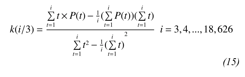
where Δt is the time interval that represents the resolution of time. In this study, Δt is equal to 2,which means three consecutive days of precipitation fluctuations. Then the slope of precipitation change during three days, k, is fitted by the least square method as follows:

The appearance probability of the precipitation series is calculated as

where Num(x) is the frequency of the occurrence of a precipitation mode x; Pkis the appearance probability of the precipitation series.

The precipitation fluctuation is divided into five equal probability intervals, and the symbols are expressed as R, r, e, d and D, respectively, which are formulated as

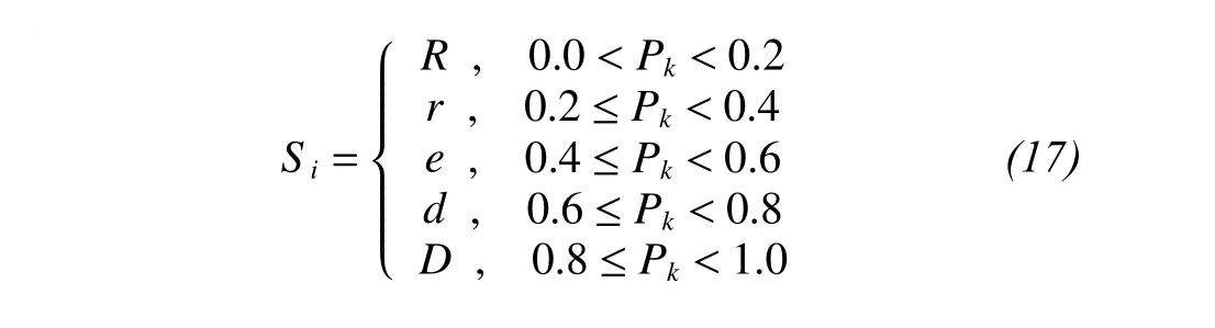
Symbols R, r, e, d and D in Formula (11) represent different meanings. R means rapidly rising, r means slowly rising, e means relatively stable, d means slowly declining, and D means fast declining, respectively. The meanings of R, r, e, d and D are illustrated in Figures 3a, 3b, 3c, 3d and 3e, respectively.

According to the above approach, the time series of daily precipitation can be translated into the symbol sequence as follows:

Repeating the above processing, we can obtain the symbol sequence for the time series of daily average temperature as follows:

Step 3: building a network. We constructed a weighted network to describe the correlation between fluctuation modes in the precipitation series. The network nodes are fluctuation modes represented by the 3-symbol strings. An edge from a node to the next node in the network represents a transition from a precipitation fluctuation mode to next one. The weight of the edge is the path number connecting the two nodes.

For example, in the precipitation fluctuation network (PFN), the symbol sequence is as follows: eRd-DeRdrdeDDDreDDDrDedDdDdedrRreeRrreRedrrD-dredDrDDedDereDdDeeRdeeRedrdeDdD, etc.. Using 3-symbol strings, {eRd, DeR, drd, eDD, Dre, DDD,rDe, dDd, Dde, drR, ree, Rrr, eRe, drr, Ddr, edD,rDD, edD, ere, DdD, eeR, dee, Red, rde, DdD, …} as the nodes of PFN, the directed connections between the nodes are as follows: eRd→DeR→drd→eDD→Dre→DDD→rDe→dDd→Dde→drR→ree→Rrr→eRe→drr→Ddr→edD→rDD→edD→ere→DdD→eeR→dee→Red→rde→DdD→….Here, we need to explain the reason for choosing 3-symbol strings such that they can better illuminate the dynamical statistics of the degrees and the distribution of degrees, clustering coefficient, the shortest path length,betweenness centrality and robustness of climate networks, compared other number of strings through a large number of empirical studies (Zhou et al., 2008;Deza et al., 2014; Sun et al., 2016; Wang and Tian,2016).

From the aforementioned steps, we constructed TFN and PFN, respectively. Figure 4a and Figure 4b show the connections between partial nodes in TFN and PFN, respectively.

Figure 4a describes the connections between the partial nodes in TFN, in which the thickness of a line connecting two nodes reflects the correlation degree between the two nodes. For example, the line between node RRR and dRR is the widest, which means that the correlation degree between the two temperature fluctuation modes represented by the two nodes (RRR and dRR) is the strongest. Figure 4b describes the connections between the partial nodes in PFN, in which the line between the node rre and err is the thickest, which indicates that the correlation degree between the two precipitation fluctuation modes represented by the two nodes (rre and err) is the strongest.

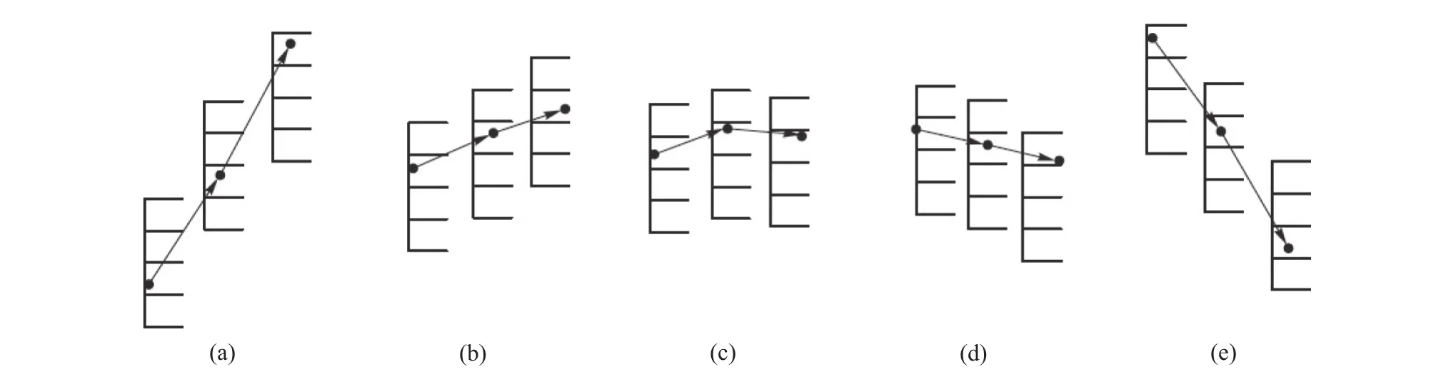
Figure 3 The meaning of symbols ((a), (b), (c), (d) and (e) means rapidly rising, slowly rising, relatively stable, slowly declining,and fast declining, respectively)

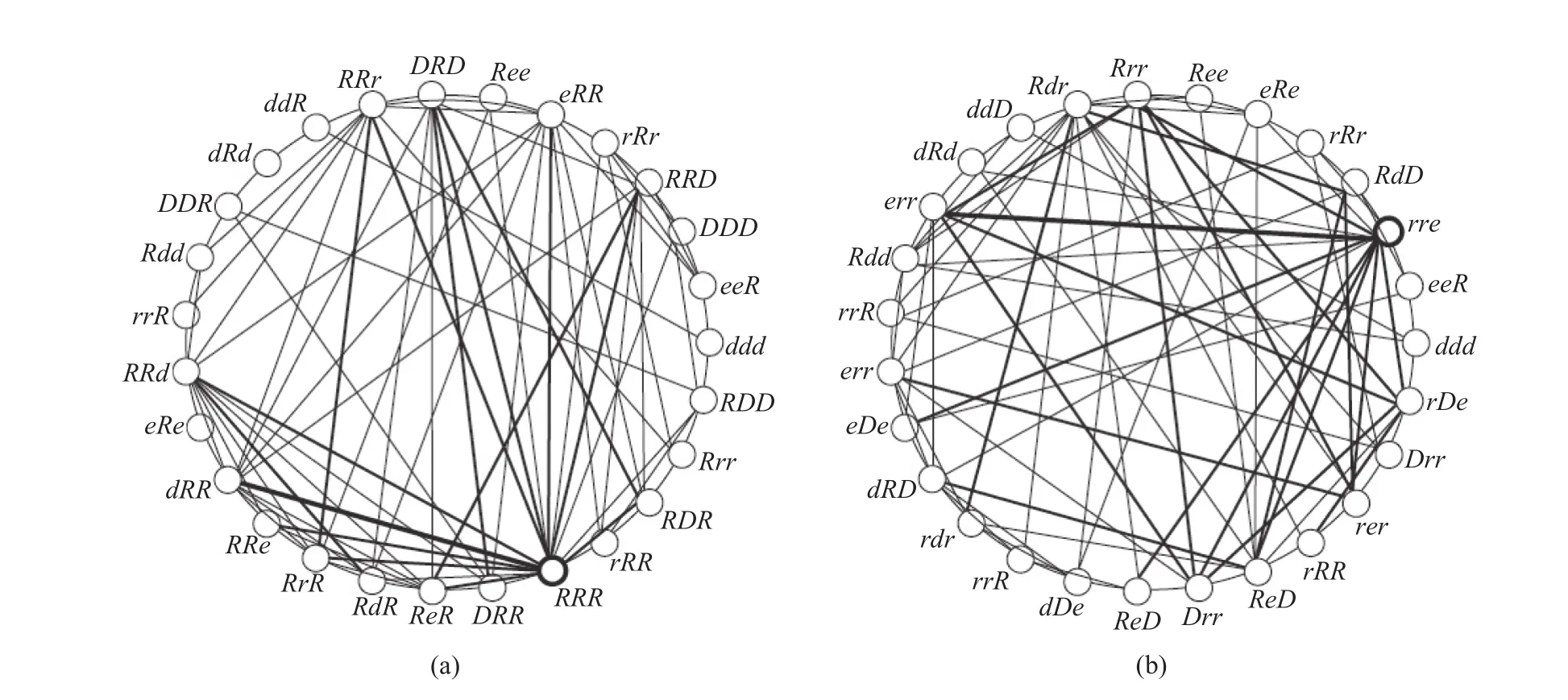
Figure 4 The connection diagram for part nodes in (a) TFN and (b) PFN

5 Results and discussion

Preparing the computing program under the Matlab environment (https://www.mathworks.com/), we calculated the degree, degree distribution, average path length, clustering coefficient and betweenness centrality for TFN and PFN. For further detailed computation, see Liu et al (2014).

Based on the computed results, we now analyze the complexity characteristics of temperature fluctuant network and precipitation fluctuant network as follows.

5.1 Degree and degree distributio n

For all the nodes in TFN and PFN except the first and end node, their in-degree and out-degree must be equal since the edges between nodes are connected in chronological order. Therefore, we only calculated the out-degree of the nodes in TFN and PFN.

Tables 1 and 2 show the node degrees of TFN and PFN, respectively. We find that nodes with big degrees in TFN are RRR, dRR, ReR and RRd, and nodes with big degrees in PFN are rre, rrr, eee and err. That is to say, these nodes are important nodes and the fluctuant modes represented by these nodes play an important role in regional climate change. This means that these fluctuate modes are frequently converted to others, or other modes are frequently converted to these important modes.

Through statistics, we found that character R frequently appears, but character D is only a few in TFN.Therefore, it is prone to rapid rise in temperature fluctuations, and extreme high temperature events are likely to occur in the Tarim River Basin. Character r in PFN appears frequently, which indicates that precipitation variation in the Tarim River Basin shows a weak increase over the past 50 years.

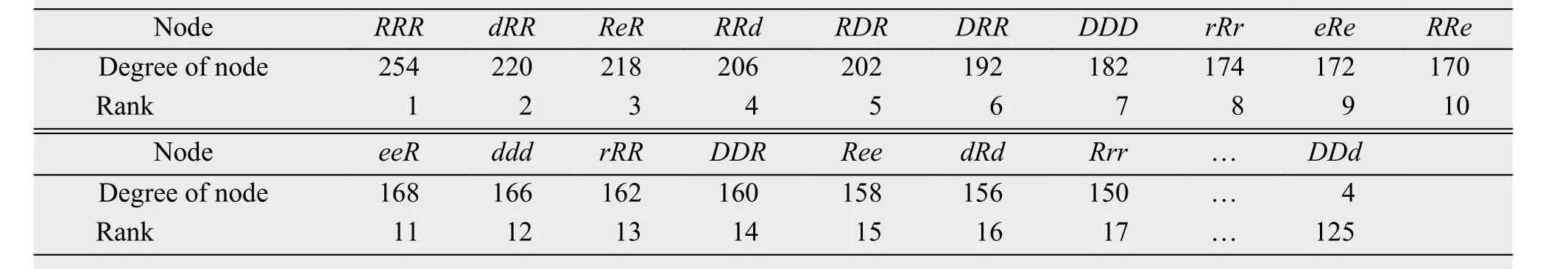
Table 1 The node degrees of TFN

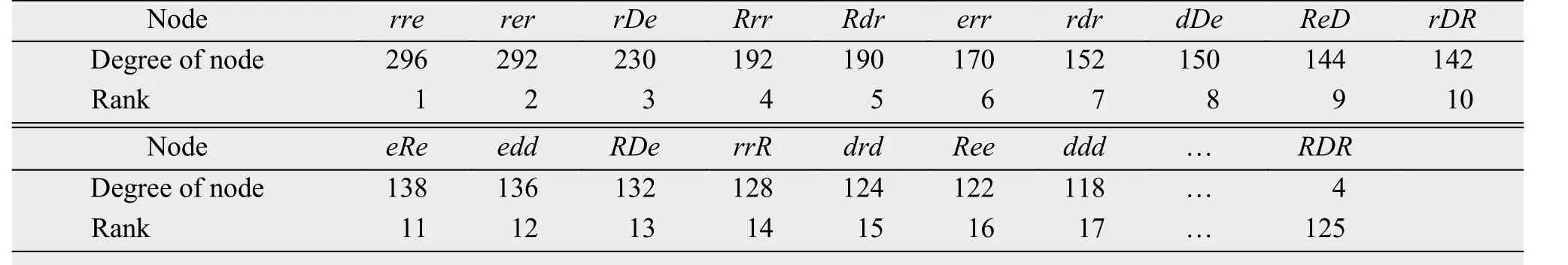
Table 2 The node degrees of PFN

Figure 5 presents the degree distribution and cumulative degree distribution of TFN and PFN. This figure shows that the degree distribution in whole or in part meets the power-law distribution with heavy tails, which is caused by random connection.

Figures 5a and 5c show the degree distribution of TFN and PFN, respectively. Figure 5a illustrates the degree distribution of TFN obeys the power law distribution of three segments, which indicates that TFN has the characteristic of scale-free, but its degree of distribution is extremely uneven. After fitting and statistical computation, we found that the two cutoff points are 60 and 100, respectively. The power exponent of the first segment is as λ1=2.038 (R2=0.992),that of the second segment is as λ2=0.198 (R2=0.956),and that of the third segment is as λ3=5.266(R2=0.941). Figure 5c illustrates that the degree distribution of PFN obeys a power law distribution, and its power exponent is as λ=2.550 (R2=0.948). These results indicate that TFN and PFN have the characteristics of a scale free network.

Figures 5b and 5d present the cumulative degree distribution of TFN and PFN, respectively, which both obey the exponential distribution of decay under the semi logarithmic coordinates. Results show that the temperature and precipitation fluctuate mode appears as certain randomness and chaotic characteristics. Although the cumulative degree distribution of TFN and PFN both obey the exponential distribution of decay, their decay rates are significantly different,which indicates that the temperature system is fast fluctuation, while the precipitation system is slow fluctuation.

5.2 Clustering coefficient and average path length

The average path length of TFN (PFN) shows the number of passed nodes in the transition from a temperature (precipitation) fluctuant mode to another. In other words, the big number of passed nodes means a long time required in the transition from a fluctuant mode to another. Therefore, the average path length reflects the average time that the transition between any two modes is required. The longer average path length indicates that the intermediate modes in the transition between any two modes are more, and the process of climate change is more complicated.

Table 3 present the clustering coefficient, average path length and average degree of nodes of TFN and PFN. The average degree of nodes of TFN is 22.6124,which indicates that the number of each node connecting to other nodes is about 23 in TFN; whereas the average degree of nodes of PFN is 85.616, which indicates that the number of each node connecting to other nodes is about 86 in PFN. The average path length of TFN is 4.523, which indicates that each node can connect to another through the transition of 3~4 times in TFN; whereas the average path length of PFN is 2.667, which indicates that each node can connect to another through the transition of 2~3 times in PFN. In addition, clustering coefficient of TFN and PFN is 0.6979 and 0.7966 respectively, which are both high. The results show that both PFN and TFN have the characteristics of scale-free networks.

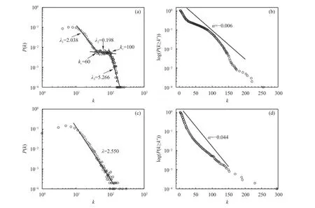
Figure 5 The degree distribution and cumulative degree distribution of TFN and PFN ((a) and (c) presents the degree distributions of TFN and PFN, respectively; (b) and (d) presents cumulative degree distribution of TFN and PFN, respectively)

Table 3 Clustering coefficient, average path length and average degree of nodes of the TFN and PFN

5.3 Betweenness centrality

Tables 4 and 5 show the rank of betweenness centrality of nodes in TFN and PFN, respectively. The betweenness centrality of nodes RRR, DDD, ReR,RRd, DDd and Ree in TFN is above 3%, and the influence of these six nodes on the whole network reached as high as 19.71%, which means that the six nodes have a pivotal role in the whole network. The betweenness centrality of nodes rre, rrr, eee and err in PFN is 3%, and the influence of these four nodes on the whole network reached is as high as 13.64%,which means that the four nodes have a pivotal role in the whole network.

6 Conclusions

Identifying these vertices of importance in topological statistics is helpful to understanding the inherent law and information transmission in a complex network. The degree, degree distribution, clustering coefficient, and average shortest path length reflect statistical properties and betweenness centrality in the heterogeneous topology of a complex network. Also in the same class system, these statistics both communicate with each other and cross inspection to a certain extent. By constructing the climate fluctuation networks and computing the network statistical metrics, this paper analyzed the complexity of climate change in the Tarim River Basin of Northwest China.

Table 4 The rank of betweenness centrality of nodes in TFN

Table 5 The rank of betweenness centrality of nodes in PFN

Summarizing the results of this study, we elicit the main conclusions as follows.

(1) The degree distribution of PFN obeys a power law distribution whereas the degree distribution of TFN obeys the power law distribution of three segments, which indicate that TFN and PFN both have the characteristics of a scale-free network. The high clustering coefficient and short average path length indicate that TFN and PFN both have the characteristics of a small-world network. In other words, both TFN and PFN have the characteristics of the scalefree network and small-world network.

(2) Nodes RRR, dRR, ReR and RRd in TFN, and nodes rre, rrr, eee and err in PFN are important modes, which indicate that the fluctuant modes represented by these nodes play an important role in regional climate change. The important nodes of TFN and PFN mostly include symbols R and r, which indicate that the variation in temperature and precipitation mainly present rising fluctuation. Therefore, it is prone to extreme heat and drought events in the Tarim River Basin.

(3) Nodes RRR, DDD, ReR, RRd, DDd and Ree in TFN are the hub nods, which undertake 19.71% of the function of betweenness centrality for the whole network. Nodes rre, rrr, eee and err in PFN are the hub nods, which undertake 13.64% of the function of betweenness centrality for whole network.

Above conclusions are of great significance in understanding the complexity of climate change in the Tarim River Basin of Northwest China.

Acknowledgments:

This work was supported by the Science and Technology Project of Jiangxi Provincial Department of Education (No. GJJ161097), the Open Foundation of the State Key Laboratory of Desert and Oasis Ecology (No. G2014-02-07), the National Natural Science Foundation of China (41630859), the Open Research Fund of Jiangxi Province Key Laboratory of Water Information Cooperative Sensing and Intelligent Processing (No. 2016WICSIP012), and the Key Project of Jiangxi Provincial Department of Science and Technology (No. 20161BBF60061).

Adamic LA, Huberman BA, Barabási AL, et al., 2000. Power-law distribution of the World Wide Web. Science, 287(5461): 2115. DOI:10.1126/science.287.5461.2115a.

Albert R, Jeong H, Barabási AL, 2000. Error and attack tolerance of complex networks. Nature, 406(6794): 378–382. DOI:10.1038/35019019.

Albert R, Barabási AL, 2002. Statistical mechanics of complex networks. Reviews of Modern Physics, 74(1): 47–97. DOI:10.1103/RevModPhys.74.47.

An F, Gao XY, Guan JH, et al., 2016. An evolution analysis of executive-based listed company relationships using complex networks.Physica A, 447: 276–285. DOI: 10.1016/j.physa.2015.12.050.

Barabási AL, Albert R, 1999. Emergence of scaling in random networks. Science, 286(5439): 509–512. DOI: 10.1126/science.286.5439.509.

Barrát A, Barthélemy M, Vespignani A, 2005. The effects of spatial constraints on the evolution of weighted complex networks. Journal of Statistical Mechanics: Theory and Experiment, 2005(5):P05003. DOI: 10.1088/1742-5468/2005/05/P05003.

Boccaletti S, Latora V, Moreno Y, et al., 2006. Complex networks:Structure and dynamics. Physics Reports, 424(4–5): 175–308. DOI:10.1016/j.physrep.2005.10.009.

Brunsell NA, 2010. A multiscale information theory approach to assess spatial-temporal variability of daily precipitation. Journal of Hydrology, 385(1–4): 165–172. DOI: 10.1016/j.jhydrol.2010.02.016.

Chen YN, Takeuchi K, Xu CC, et al., 2006. Regional climate change and its effects on river runoff in the Tarim Basin, China. Hydrological Processes, 20(10): 2207–2216. DOI: 10.1002/hyp.6200.

Deza JI, Masoller C, Barreiro M, 2014. Distinguishing the effects of internal and forced atmospheric variability in climate networks.Nonlinear Processes in Geophysics, 21(3): 617–631. DOI:10.5194/npg-21-617-2014.

Du HB, Wu ZF, Li M, et al., 2013. Characteristics of extreme daily minimum and maximum temperature over Northeast China,1961–2009. Theoretical and Applied Climatology, 111(1–2):161–171. DOI: 10.1007/s00704-012-0649-3.

Faloutsos M, Faloutsos P, Faloutsos C, 1999. On power-law relationships of the internet topology. ACM Sigcomm Computer Communication Review, 29(4): 251–262. DOI: 10.1145/316194.316229.

Fan QB, Wang YX, Zhu L, 2013. Complexity analysis of spatial-temporal precipitation system by PCA and SDLE. Applied Mathematical Modelling, 37(6): 4059–4066. DOI: 10.1016/j.apm.2012.09.009.

Fan ZM, Yue TX, Chen CF, et al., 2011. Spatial change trends of temperature and precipitation in China. Journal of Geo-Information Science, 13(4): 526–533. DOI: 10.3724/SP.J.1047.2011.00526.

Feldhoff JH, Lange S, Volkholz J, et al., 2015. Complex networks for climate model evaluation with application to statistical versus dynamical modeling of South American climate. Climate Dynamics,44(5–6): 1567–1581. DOI: 10.1007/s00382-014-2182-9.

Fraedrich K, 1986. Estimating the dimensions of weather and climate attractors. Journal of the Atmospheric Sciences, 43(5): 419–432.DOI: 10.1175/1520-0469(1986)043<0419:ETDOWA>2.0.CO;2.

Hossain MM, Alam S, 2017. A complex network approach towards modeling and analysis of the Australian airport network. Journal of Air Transport Management, 60: 1–9. DOI: 10.1016/j.jairtraman.2016.12.008.

Katz RW, Brown BG, 1992. Extreme events in a changing climate:Variability is more important than averages. Climatic Change,21(3): 289–302. DOI: 10.1007/BF00139728.

Li BF, Chen YN, Shi X, et al., 2013. Temperature and precipitation changes in different environments in the arid region of northwest China. Theoretical and Applied Climatology, 112(3–4): 589–596.DOI: 10.1007/s00704-012-0753-4.

Li QH, Chen YN, Shen YJ, et al., 2011a. Spatial and temporal trends of climate change in Xinjiang, China. Journal of Geographical Sciences, 21(6): 1007–1018. DOI: 10.1007/s11442-011-0896-8.

Li XM, Jiang FQ, Li LH, et al., 2011b. Spatial and temporal variability of precipitation concentration index, concentration degree and concentration period in Xinjiang, China. International Journal of Climatology, 31(11): 1679–1693. DOI: 10.1002/joc.2181.

Liljeros F, Edling CR, Amaral LAN, et al., 2001. The web of human sexual contacts. Nature, 411(6840): 907–908. DOI: 10.1038/35082140.

Liston GE, Pielke RA, 2000. A climate version of the regional atmospheric modeling system. Theoretical and Applied Climatology,66(1–2): 29–47. DOI: 10.1007/s007040070031.

Liu ML, Adam JC, Hamlet AF, 2013. Spatial-temporal variations of evapotranspiration and runoff/precipitation ratios responding to the changing climate in the Pacific Northwest during 1921–2006.Journal of Geophysical Research: Atmospheres, 118(2): 380–394.DOI: 10.1029/2012JD018400.

Liu ZH, 2014. A Study of the Complex and Nonlinear Investigation of Climatological-Hydrological Process in the Tarim River Basin.Shanghai: East China Normal University, Doctoral thesis, pp.287–291.

Liu ZH, Wang LL, Yu X, et al., 2017. Multi-scale response of runoff to climate fluctuation in the headwater region of the Kaidu River in Xinjiang of China. Atmospheric Science Letters, 18(5): 230–236.DOI: 10.1002/asl.747.

Liu ZH, Xu JH, Shi K, 2014a. Self-organized criticality of climate change. Theoretical and Applied Climatology, 115(3–4): 685–691.DOI: 10.1007/s00704-013-0929-6.

Liu ZH, Xu JH, Chen ZS, et al., 2014b. Multifractal and long memory of humidity process in the Tarim River Basin. Stochastic Environmental Research and Risk Assessment, 28(6): 1383–1400. DOI:10.1007/s00477-013-0832-9.

Livada I, Charalambous G, Assimakopoulos MN, 2008. Spatial and temporal study of precipitation characteristics over Greece. Theoretical and Applied Climatology, 93(1–2): 45–55. DOI:10.1007/s00704-007-0331-2.

Lorenz EN, 1991. Dimension of weather and climate attractors. Nature,353(6341): 241–244. DOI: 10.1038/353241a0.

Lymperopoulos IN, Ioannou GD, 2016. Understanding and modeling the complex dynamics of the online social networks: a scalable conceptual approach. Evolving Systems, 7(3): 207–232. DOI:10.1007/s12530-016-9145-9.

Martínez MD, Lana X, Burgueño A, et al., 2007. Spatial and temporal daily rainfall regime in Catalonia (NE Spain) derived from four precipitation indices, years 1950–2000. International Journal of Climatology, 27(1): 123–138. DOI: 10.1002/joc.1369.

Maslov S, Sneppen K, 2002. Specificity and stability in topology of protein networks. Science, 296(5569): 910–913. DOI: 10.1126/science.1065103.

McLuhan M, 1964. Understanding Media: The Extensions of Man.New York: McGraw Hill.

Meng X, Shen EH, Chen F, et al., 2000. Coarse graining in complexity analysis of EEG: I. Over coarse graining and a comparison among three kinds of complexities. Acta Biophysica Sinica, 16(4):701–706. DOI: 10.3321/j.issn:1000-6737.2000.04.007.

Millán H, Kalauzi A, Llerena G, et al., 2009. Meteorological complexity in the Amazonian area of Ecuador: An approach based on dynamical system theory. Ecological Complexity, 6(3): 278–285.DOI: 10.1016/j.ecocom.2009.05.004.

Montoya JM, Pimm SL, Solé RV, 2006. Ecological networks and their fragility. Nature, 442(7100): 259–264. DOI: 10.1038/nature04927.

Newman MEJ, 2001. Clustering and preferential attachment in growing networks. Physical Review E, 64(2): 025102. DOI:10.1103/PhysRevE.64.025102.

Newman MEJ, 2010. Networks: An Introduction. Oxford, UK: Oxford University Press.

Nie Q, Xu JH, Li Z, et al., 2012. Spatial-temporal variations of vegetation cover in Yellow River Basin of China during 1998–2008. Sciences in Cold and Arid Regions, 4(3): 211–221. DOI:10.3724/SP.J.1226.2012.00211.

Palmer TN, 1999. A nonlinear dynamical perspective on climate prediction. Journal of Climate, 12(2): 575–591. DOI: 10.1175/1520-0442(1999)012<0575:ANDPOC>2.0.CO;2.

Palmer TN, 2000. Predicting uncertainty in forecasts of weather and climate. Reports on Progress in Physics, 63(2): 71–116. DOI:10.1088/0034-4885/63/2/201.

Pasten D, Abe S, Muñoz V, et al., 2010. Scale-free and small-world properties of earthquake network in Chile. arXiv Preprint arXiv:1005.5548.

Ray A, 2004. Symbolic dynamic analysis of complex systems for anomaly detection. Signal Processing, 84(7): 1115–1130. DOI:10.1016/j.sigpro.2004.03.011.

Rendón de la Torre S, Kalda J, Kitt R, et al., 2016. On the topologic structure of economic complex networks: Empirical evidence from large scale payment network of Estonia. Chaos, Solitons &Fractals, 90: 18–27. DOI: 10.1016/j.chaos.2016.01.018.

Rezvanian A, Meybodi MR, 2016. Stochastic graph as a model for social networks. Computers in Human Behavior, 64: 621–640. DOI:10.1016/j.chb.2016.07.032.

Rial JA, Pielke RA, Beniston M, et al., 2004. Nonlinearities, feedbacks and critical thresholds within the Earth's climate system. Climatic Change, 65(1–2): 11–38. DOI: 10.1023 B:CLIM.0000037493.89489.3f.

Rodriguez-Iturbe I, De Power FB, Sharifi MB, et al., 1989. Chaos in rainfall. Water Resources Research, 25(7): 1667–1675. DOI:10.1029/WR025i007p01667.

Saha M, Mitra P, 2015. Climate network based index discovery for prediction of Indian monsoon. In: Kryszkiewicz M, Bandyopadhyay S, Rybinski H, et al. (eds.). Pattern Recognition and Machine Intelligence. Cham: Springer, pp. 554–564. DOI: 10.1007/978-3-319-19941-2_53.

Steinhaeuser K, Ganguly AR, Chawla NV, 2009. Complex networks as a tool of choice for improving the science of climate extremes and reducing uncertainty in their projections. In: AGU Fall Meeting Abstracts. Washington D.C. American Geophysical Union.

Steinhaeuser K, Chawla NV, Ganguly AR, 2011. Complex networks as a unified framework for descriptive analysis and predictive modeling in climate science. Statistical Analysis and Data Mining, 4(5):497–511. DOI: 10.1002/sam.10100.

Sun LN, Liu ZH, Wang JY, et al., 2016. The evolving concept of air pollution: a small-world network or scale-free network? Atmospheric Science Letters, 17(5): 308–314. DOI: 10.1002/asl.659.

Tirabassi G, Masoller C, 2016. Unravelling the community structure of the climate system by using lags and symbolic time-series analysis.Scientific Reports, 6: 29804. DOI: 10.1038/srep29804.

Tsonis AA, Elsner JB, 1988. The weather attractor over very short timescales. Nature, 333(6173): 545–547. DOI: 10.1038/333545a0.

Vázquez A, Pastor-Satorras R, Vespignani A, 2002. Large-scale topological and dynamical properties of the Internet. Physical Review E, 65(6): 066130. DOI: 10.1103/PhysRevE.65.066130.

Wang MG, Tian LX, 2016. From time series to complex networks: The phase space coarse graining. Physica A, 461: 456–468. DOI:10.1016/j.physa.2016.06.028.

Watts DJ, Strogatz SH, 1998. Collective dynamics of 'small-world' networks. Nature, 393(6684): 440–442. DOI: 10.1038/30918.

Wiedermann M, Radebach A, Donges JF, et al., 2016. A climate network-based index to discriminate different types of El Niño and La Niña. Geophysical Research Letters, 43(13): 7176–7185. DOI:10.1002/2016GL069119.

Xu JH, Chen YN, Li WH, et al., 2009. Wavelet analysis and nonparametric test for climate change in Tarim River Basin of Xinjiang during 1959–2006. Chinese Geographical Science, 19(4): 306–313.DOI: 10.1007/s11769-009-0306-7.

Xu JH, Li WH, Ji MH, et al., 2010. A comprehensive approach to characterization of the nonlinearity of runoff in the headwaters of the Tarim River, western China. Hydrological Processes, 24(2):136–146. DOI: 10.1002/hyp.7484.

Xu JH, Chen YN, Li WH, et al., 2011a. An integrated statistical approach to identify the nonlinear trend of runoff in the Hotan River and its relation with climatic factors. Stochastic Environmental Research and Risk Assessment, 25(2): 223–233. DOI:10.1007/s00477-010-0433-9.

Xu JH, Chen YN, Lu F, et al., 2011b. The nonlinear trend of runoff and its response to climate change in the Aksu River, western China. International Journal of Climatology, 31(5): 687–695. DOI:10.1002/joc.2110.

Xu JH, Chen YN, Li WH, et al., 2013a. The nonlinear hydro-climatic process in the Yarkand River, northwestern China. Stochastic Environmental Research and Risk Assessment, 27(2): 389–399. DOI:10.1007/s00477-012-0606-9.

Xu JH, Chen YN, Li WH, et al., 2013b. Understanding the complexity of temperature dynamics in Xinjiang, China, from multitemporal scale and spatial perspectives. The Scientific World Journal, 2013:259248. DOI: 10.1155/2013/259248.

Xu JH, Chen YN, Li WH, et al., 2013c. Combining BPANN and wavelet analysis to simulate hydro-climatic processes–a case study of the Kaidu River, Northwest China. Frontiers of Earth Science,7(2): 227–237. DOI: 10.1007/s11707-013-0354-2.

Xu JH, Chen YN, Li WH, et al., 2014a. Integrating wavelet analysis and BPANN to simulate the annual runoff with regional climate change: a case study of Yarkand River, northwest China. Water Resources Management, 28(9): 2523–2537. DOI: 10.1007/s11269-014-0625-z.

Xu JH, Li WH, Hong YL, et al., 2014b. A quantitative assessment on groundwater salinization in the Tarim River lower reaches, Northwest China. Sciences in Cold and Arid Regions, 6(1): 44–51. DOI:10.3724/SP.J.1226.2014.00044.

Xu JH, Chen YN, Li WH, et al., 2016a. Understanding temporal and spatial complexity of precipitation distribution in Xinjiang, China.Theoretical and Applied Climatology, 123(1–2): 321–333. DOI:10.1007/s00704-014-1364-z.

Xu JH, Chen YN, Bai L, et al., 2016b. A hybrid model to simulate the annual runoff of the Kaidu River in northwest China. Hydrology and Earth System Sciences, 20(4): 1447–1457. DOI: 10.5194/hess-20-1447-2016.

Zeng X, Pielke RA, Eykholt R, 1992. Estimating the fractal dimension and the predictability of the atmosphere. Journal of the Atmospheric Sciences, 49(8): 649–659. DOI: 10.1175/1520-0469(1992)049<0649:ETFDAT>2.0.CO;2.

Zhou L, Gong ZQ, Zhi R, et al., 2008. An approach to research the topology of Chinese temperature sequence based on complex network. Acta Physica Sinica, 57(11): 7380–7389. DOI: 10.3321/j.issn:1000-3290.2008.11.111.

: Liu ZH, Xu JH, Li WH, 2017. Complex network analysis of climate change in the Tarim River Basin, Northwest China. Sciences in Cold and Arid Regions, 9(5): 0476–0487.

10.3724/SP.J.1226.2017.00476.

*Correspondence to: JianHua Xu, Professor, Key Laboratory of Geographic Information Science (Ministry of Education),School of Geographic Sciences, East China Normal University. No. 500 Dongchuan Road, Shanghai 200241, China.E-mail: jhxu@geo.ecnu.edu.cn

February 27, 2017 Accepted: April 28, 2017