YIN Feng(印 峰), CHEN Xinyu(陈新雨), QIU Jie(邱 杰), KANG Yongliang(康永亮)

1 College of Automation and Electronic Information, Xiangtan University, Xiangtan 411105, China 2 National Engineering Laboratory of Robot Vision Perception and Control Technology, Changsha 410012, China

Abstract: Boundary equilibrium generative adversarial networks (BEGANs) are the improved version of generative adversarial networks (GANs). In this paper, an improved BEGAN with a skip-connection technique in the generator and the discriminator is proposed. Moreover, an alternative time-scale update rule is adopted to balance the learning rate of the generator and the discriminator. Finally, the performance of the proposed method is quantitatively evaluated by Fréchet inception distance (FID) and inception score (IS). The test results show that the performance of the proposed method is better than that of the original BEGAN.

Key words: generative adversarial network (GAN); boundary equilibrium generative adversarial network (BEGAN); Fréchet inception distance (FID); inception score (IS)

Introduction

As one kind of methods for generating models, generative adversarial networks (GANs)[1]excel at generating realistic images[2-4], creating videos[5-7]and producing text[8-9]. The architecture of GANs composed of two subnetworks is a deep convolutional neural net. One subnetwork is used as a generator to synthesize data from random noise. The other is used as a discriminator to separate above synthesized data (also known as fake data) from real data. The competition between the generator and the discriminator drives both to improve themselves until the counterfeits are indistinguishable from real data. As a powerful subclass of generative models, GANs have achieved great success in many fields such as semi-supervised learning[10], semantic segmentation[11], small object detection[12]and so on. However, it cannot perform very well on some practical issues. In general, it is very hard to effectively train GANs without additional auxiliaries because of high need for well-designed network structures and hyper-parameters. There have been many different attempts to solve these issues mainly from three perspectives.

The first attempt is the improvement of the object functions. Nowozinetal.[13]noticed that not just Jensen-Shannon (JS) divergence, any divergence can be placed in the GAN architecture. Least-square GAN (LSGAN)[14]replaces sigmoid cross entropy loss in the standard GAN with least square loss, which can improve the quality of picture generation and make the training stable by directly moving generator samples close to real data distribution. Wasserstein GAN (WGAN)[15]introduces Earth-Mover (EM) distance which has superior smoothing characteristics with respect to relative Kullback-Leibler (KL) divergence and JS divergence. The EM distance used as a cost function not only solves the problem of unstable training, but also provides a reliable training process indicator. WGAN-gradient penalty (WGAN-GP) is an improved version of WGAN. The approximate 1-Lipschitz limit on the discriminator is achieved with gradient penalty. WGAN-GP achieves very good results in the further test.

The second attempt is the modification of the network structure. Well-architected generators and discriminators are more important for GANs. The most commonly used structure is convolutional neural networks (CNNs) in the image processing field[2]. The core idea of the approach in Ref. [2] is adopting and modifying demonstrated changes to CNN architectures. Experiments show that deep convolution generative adversarial networks (DCGANs) can provide a high quality generation process. Especially, it is very good at solving semi-supervised classification tasks. Self-attention generative adversarial networks (SAGANs)[4]use the self-attention paradigm to capture long-range spatial relationships that exist in images to better synthesize new images. Under good hardware with a tensor processor unit (TPU) and huge parameter system conditions, large scale GAN training for high fidelity natural image synthesis (denoted by BigGAN)[16]increases batch size and channel to produce realistic sharp pictures.

The third attempt is the use of additional networks or supervision conditions. In addition to the different cost function and network framework, additional networks or supervision conditions are often adopted to further improve the performance of GANs. It is interesting to note that the architecture of the generator in GANs does not differ significantly from other approaches like variational auto-encoders (VAEs)[17]. VAEs, GANs and their variants are three kinds of generation models based on deep learning. It is normal practice to combine GANs with auto-encoder networks, such as VAE-GANs[18]and energy-based GANs (EBGANs)[19]. Compared with using the VAE alone, the VAE-GAN combining VAEs and GANs can produce clearer pictures. In the VAE-GAN, one discriminator is used to authenticate the input image whether it is from real data or generated samples. In contrast, the discriminator used in the EBGAN is adopted to identify the re-configurability of the input image. That is it can remember what real data distribution looks like and then give a high score as long as the arbitrary inputxis close to that of the real sample. In other improved methods of GANs, supervision conditions are added. In conditional generative adversarial nets (CGANs), an additional condition variable is introduced into both of the generator and the discriminator. The involved information can be used to guide the data generation process in the CGAN[20]. The information maximizing GAN (Info-GAN) contains a hidden variablecwhich is also known as the latent code. By associating latent code and generated data with additional constrains, letccontain interpretable information about the data to help Info-GAN[21]find an interpretable expression. Warde-Farley and Bengio[22]proposed a denoising feature matching (DFM) technique to guide the generator toward probable configurations of abstract discriminator features. A de-noising auto-encoder is used to greatly improve the GAN image model.

In this paper, we proposed an improved BEGAN with a skip-connection technique in the generator and the discriminator. The use of the skip-connection technique allows feature information to be transmitted directly across layers. Its greatest advantage is that it can reduce the information loss in the process of transmission. More feature information can improve the performance of generated images. Moreover, an alternative time-scale update rule was proposed to balance the learning rates of the generator and the discriminator. As a result, more realistic pictures can be generated by using the proposed method. Finally, we evaluated the performance of the proposed method, and compared it with BEGANs[23], improving generative adversarial networks with DFM[22], adversarial learned inference (ALI)[24], improved techniques for training GANs (Improved GANs)[25]and generalization and equilibrium in generative adversarial nets (denoted by MIX+WGAN)[26].

1 Review of Generative Adversarial Networks

A GAN involves generator networks and discriminator networks whose purposes are to map random noise to samples and discriminate real and generated samples, respectively[16]. LetGθdenote the generator with the parametersθandDφdenote the discriminator with the parameterφ. Formally, the GAN objective, in its original form, involves finding Nash equilibrium for the following two-player min-max problem until neither player can improve its cost unilaterally. Both players aim to minimize their own cost function. The cost function for the discriminator is defined as

(1)

where the distributions of real dataxand random noisezarep(x) andp(z), respectively. In the minimax GAN, the discriminator (shown in Eq.(1)) attempts to classify generated images (fake images) from real images and outputs a probability. Simultaneously, the generator attempts to fool the discriminator and learns to generate samples that have a low probability of judging fake. The cost function for the generator in minimax the GAN is defined as

(2)

To improve the gradient, Goodfellowetal.[1]also proposed a non-saturating GAN as an alternative cost function, where the generator instead aims to maximize the probability of generated samples being real[27]. The cost function for the generator in the non-saturating GAN is defined as

(3)

The original GAN adopts the JS divergence to measure the distance between the distribution of real data and random noise. It is noted that the generation model and the discriminant model can be various neural networks without any limitations. During the training process of the GAN, the goals of the discriminator and the generator training are just opposite. The former is to maximize the discriminative accuracy to better distinguish between the real data and the generated data. In contrast, the latter is to minimize the discriminant accuracy of the discriminator. Generally, without auxiliary stabilization techniques, training procedure of GANs is notoriously brittle.

2 Proposed Methods and Architectures

Under the condition of the near-optimal discriminator, minimization of the loss of the generator is equivalent to minimizing the JS divergence betweenp(x) andp(z). In practice, the distributions of both are almost impossible to have substantial overlap, which eventually cause the gradient of the generator close to 0. In other words, the gradient disappears. This problem can be alleviated to some extent by an alternative non-saturating cost function. The minimization of the cost function is equivalent to minimizing an unreasonable distance measurement. However, there are also two problems to be solved: one is gradient instability, and the other is mode collapse.

WGANs[15], BEGANs[23]and SAGANs[4]are excellent methods proposed to solve above problems. WGANs suggest the EM distance, also called the Wasserstein distance, as a measure of the discrepancy between two distributions. BEGANs adopt the distances between loss distributions, instead of sample distributions. A self-attention mechanism is added into the SAGAN. Moreover, the spectral normalization and two time-scale update rule (TTUR) optimization techniques are used to stabilize GAN training. Next, we will develop an improved BEGAN. The proposed BEGAN based network is shown in Fig. 1. The generator and the discriminator both adopt an encoder-decoder framework. Between them, the architecture of the discriminatorDis a deep convolutional neural network.Nxis short for the dimensions ofx.Nx=H×W×C, whereH,WandCare height, width and color, respectively; for RGB images,C=3. The architecture of the generatorGhas the dimensions ofH×W×C.Guses the same architecture as the decoder of the discriminator. The generator network illustrated in the upper section of Fig. 1 contains nine convolutional layers and three up-sampling convolutional layers.

Fig. 1 Architectures of the generator networks and the discriminator networks with convolutional kernel size and output channels for each convolutional layer (SL denotes the skip layer; Conv w=(k, k) denotes a convolutional layer with k×k kernel; in d=(a, b), a and b denote input and output filters, respectively; n denotes the number of filters/channels)

It is noted that the proposed method also uses the auto-encoder as the discriminator and aims to match the auto-encoder loss distributions using a loss derived from the Wasserstain distance. The definitions of the Wasserstain distance and its lower bound are stated as follows.

LetL(ν)=|ν-D(ν)|η, whereη∈{1, 2}, and it is the target norm. LetΓ(u1,u2) be the set all of couplings ofu1andu2, whereu1andu2are two distributions of auto-encoder losses. Letm1andm2be their respective means, wherem1∈R andm2∈R. The Wasserstain distance can be confirmed as

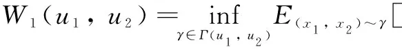
(4)

By taking Jensen’s inequality, the lower bound ofW1(u1,u2)can be derived as

infE[|x1-x2|]≥inf|E[x1-x2]|=|m1-m2|.

(5)

Letu1be the distribution of real data losses andu2be the distribution of the lossL(G(z)). Equation (5) shows that the infimum ofW1(u1,u2) is|m1-m2|.

In order to maximize the distance between real data and generated data auto-encoder losses, there are only two solutions to maximize|m1-m2|ofW1(u1,u2)≥m1-m2, wherem1→∞andm2→0, orW1(u1,u2)≥m2-m1, wherem1→0 andm2→∞. Therefore minimizingm1naturally leads to auto encoding the real images. Similar to the BEGAN, the objective of the network training is to meet

(6)

where,L(x)is the auto-encoder loss of real data, andL(x)=D(x)-x;L(G(zD)) is the auto-encoder loss of generated data, andL(G(zD))=D(G(zD))-G(zD); a variablektis used to control how much emphasis is placed on generator losses during gradient descent and initializek0in this work, andkt∈[0, 1];λkis the learning rate ofkt; the hyper-parameterγ=E[|L(G(z))|]/E[|L(x)|]∈[0, 1] , balances these two goals, namely auto-encoder real images and discriminate real images from generated images, and at the same time,γis also an indicator about image diversity where a lower value means lower image diversity. Deriving a global measure of convergence is formulated as the sum of these two terms:

Mglobal=L(x)+|γL(x)-L(G(zG))|,

(7)

where lowerMglobalmeans better training process. Figure 2 shows the detail process of image generation. To generate more real images, we would like to use Algorithm 1 to converge to a good estimator ofpdataif given enough capacity and training time, and Adam stands for adaptive moment estimation.

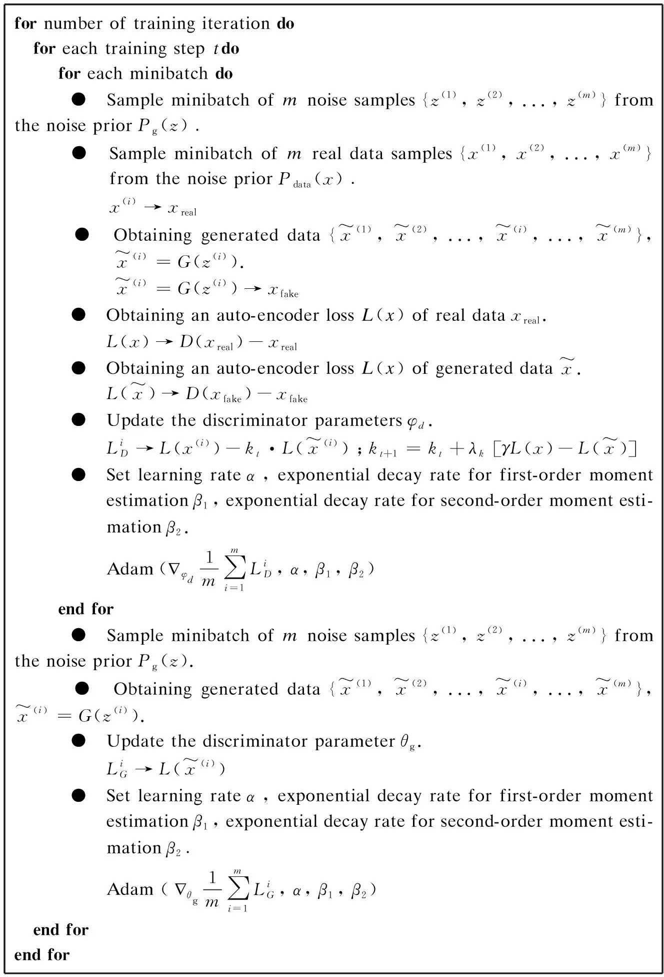
Fig. 2 Detail process of image generation

When applying the GAN, it is required that the discriminating ability of the discriminator is better than the generating ability of the current generator. To achieve this aim, the usual practice is to update the parameters of the discriminator more times than the generator during training. It is noted that the discriminator often learns faster than the generator in practice. To balance the learning speed, the TTUR[28]is adopted during the training process. Specifically, a same update rate but different learning rates are adopted in the TTUR when training the discriminator and the generator. As they have the same update rate, we only need to adjust the learning rate. Here, the learning rate is set to be 0.004 and 0.001 respectively for the discriminator and generator training. It is because choosing a relatively high learning rate can accelerate the learning speed of the discriminator. And a small learning rate is necessary for the generator to successfully fool the discriminator.

Furthermore, a strategy of adding skip connection[29]between different layers is applied to strengthen feature propagation and encourage the reuse of feature. The feature information can be directly transmitted across layers with the help of additional skip connection. Then the integrity of the feature is preserved to the greatest extent. The skip-connection structure adopted in our model is that the input is additionally connected to the output for each convolution block. These skip connection is only added into the generator and the decoder. It is noted that another structure of skip connection similar to dense block is mentioned in the BEGAN. By comparison, our structure is more suitable for processing big dataset because of its simple connection. The data flow diagram of the generator and the discriminator in our model is shown in Fig. 3.

Fig. 3 Data flow diagram of the generator and the discriminator (L(·) denotes auto-encoder loss)

3 Experiments

In this section, a series of experiments were conducted to demonstrate the performance of the proposed method.

3.1 Parameter settings

The architecture of the model is shown in Fig. 1. Both the discriminator and the generator use 3×3 convolutions with exponential liner units (ELUs) activation function for outputs. Many of these convolution layers constitute a convolution block. Specifically, two layers are used in this paper. The training of the generator and the discriminator both include down-sampling and up-sampling phases. Down-sampling is implemented as sub-sampling with stride 2 and sub-sampling is done by the nearest neighbour. The learning approach adopts Adam optimization algorithm with the initial learning rate of 0.000 1. Note that the learning rate will be adjusted by multiplying a factor of 2 when convergence stalls. The batch size, one of the important parameters, is set to be 16. The sizes of input images are 64×64. Note that the model is also suitable for varied resolution from 32 to 256 by adjusting convolution layers while keeping 8×8 size of the final down-sampled image.

All training processes are conducted on a NVIDIA GeForce GTX 1080Ti GPU using 162 770 face images, randomly sampled from the large-scale celeb faces attributes (CelebA), and 60 000 images of 10 categories from CIFAR-10. Training images are different from the testing images.

3.2 Computational experiments

In this example, the data set used is CelebA with a larger variety of facial poses. It is noted that we resize the images to 64×64 to highlight the areas where faces are located in images. We prefer to do this since humans are better at identifying flaws appearing on the faces. First, we discuss the effect of another hyper-parameterγ∈{0, 1} and perform several group comparison tests. The value ofγis related to the quality and the diversity of the generated images. As shown in Fig. 4, we can observe skin colour, expression, moustaches, gender, hair colour, hair style and age from the generated images.

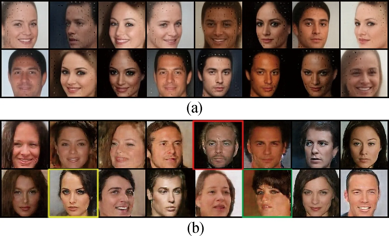
Fig. 4 Comparison of samples randomly generated under different γ : (a) γ=0.3; (b) γ=0.7

In order to observe the influence ofγconveniently, we change its values across the range [0, 1] in tests. Some typical results about image diversity are displayed in Fig. 4. Overall, the generated images appear to be well behaved. When the parameter is at a lower level, such asγ=0.3, the generated images look overly uniform, and contain more noise. The facial contours are gradually becoming similar, and the generated face samples are drawn to less diverse. Moreover, the noises are greatly reduced. From Fig. 4(a), it can be seen that little noises are concentrated around the picture, such as positions located near the hair and forehead. What’s more, more detailed features can be created successfully, like beards, blue eyes and bangs highlighted in Fig. 4(b). Note that these features are usually hard to be created by other methods.

Furthermore, we quantitatively evaluate the performance of the proposed method. In this paper, a widely used quantitative measurement method, Fréchet inception distance (FID), is adopted for evaluation. The FID[28]provides a more principled and comprehensive metric. It compares the distributions between the generated images and real images in the feature space of inception networks. Lower FID means closer distances between synthetic and real date distributions. Figure 5 shows a series of 64×64 random generated samples based on the proposed method. From the visual point of view, the generated images are very impressive. It can even generate teeth images clearly.

Fig. 5 Random generated samples (γ=0.5)

It can be seen from Fig. 6 that the FID of our model decreases sharply at the beginning of the iteration, and gradually decreases with a mild concussion. By comparison, the FID value of the BEGAN fluctuates greatly, and suddenly increases dramatically in the late stages of the iteration. Figure 7 shows the convergence curves of theLD. The results show that our method is slightly better. Moreover, the numerical results show that FID values obtained based on BEGANs and our model are 84.19 and 24.57, respectively. At this point, the performance of our method increases by 3.4 times.

Fig. 6 Comparison of the BEGAN and our model about convergence curves of the FID in CelebA datasets

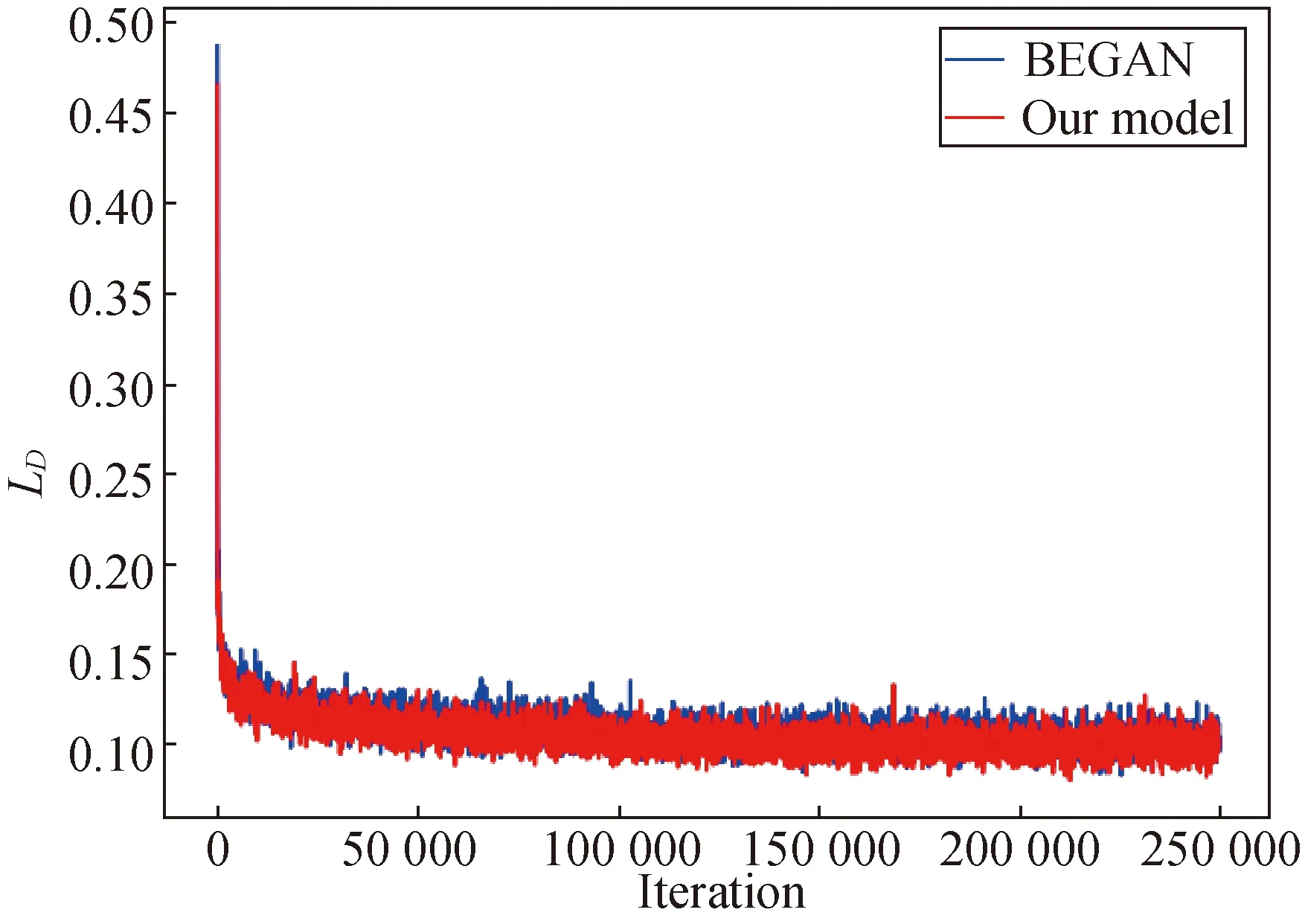
Fig. 7 Comparison of the BEGAN and our model about convergence curves of LD in CelebA datasets

Another dataset used in the test is the fashion MNIST dataset, which consists of a training set of 60 000 samples and a test set of 10 000 samples. Unlike the previous CelebA dataset, the samples in the fashion MNIST dataset is a grayscale image, associated with a label from 10 classes. The parameters are set as follows: the size of the input images is 32×32, the batch size is 64 and the iteration number is 100 000.

Figure 8 shows some results of generated random samples based on the proposed method. As can be seen from Fig. 8, a variety of shoe styles can be successfully generated.

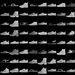
Fig. 8 Random samples generated on the fashion MNIST dataset (the picture contains a variety of shoe styles)

Furthermore, we compare FID and inception score (IS) of the BEGAN and our model. IS is another widely used quantitative measurement to evaluate the performances of the comparing methods[25]. It uses an inception network pre-trained on ImageNet to compute the KL-divergence between the conditional class distribution and the marginal class distribution. Higher IS indicates better image quality and diversity.

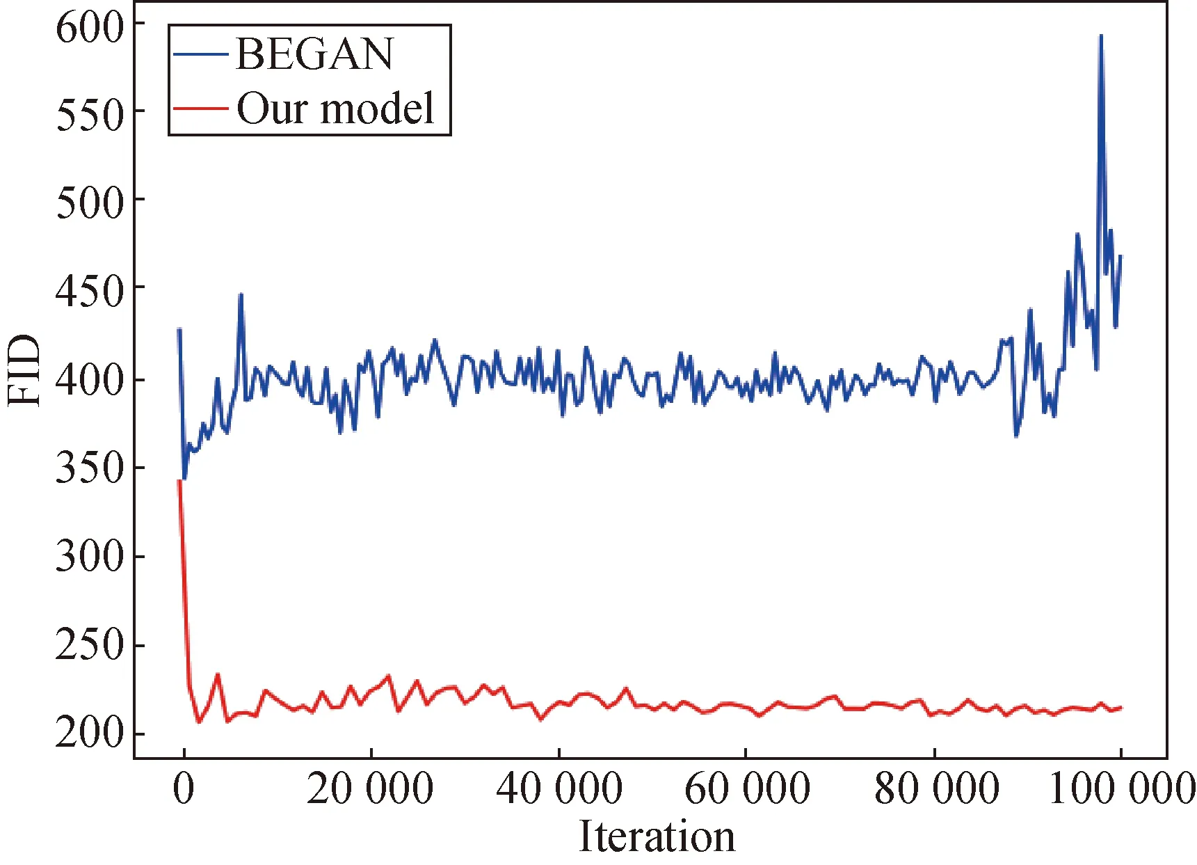
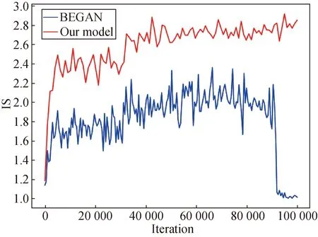
As can be seen from Fig. 9(a), the FID of our model is significantly smaller than that of the BEGAN. According to the analysis above, the quality of the images generated by our model is higher. Figure 9(b) shows the results of IS. It can be seen that higher IS can be obtained by our model. Moreover, the IS shows an upward trend at 100 000 iteration.

(a)

(b)

Fig. 9 Comparison of (a) FID and (b) IS of the BEGAN and our model in the fashion MNIST dataset

4 Verification

In this section, we further compare the performances among the proposed method and common classical methods, including BEGANs, ALIs, DFMs, Improved GANs and MIX+WAGN. In these comparison experiments, we retrain models on the single NVIDIA GeForce GTX 1080 Ti GPU with CIFAR-10 dataset, which goes through 100 000 iterations and the batch size is 64. The values of other hyper-parameters are defaults as in the train file. All models are built based on TensorFlow.

The used dataset is CIFAR-10. We calculate IS of the comparing methods with an average of 10 evaluations for 50 000 samples. The final numerical results are shown in Table 1. The test results show that our score is better than all methods except for the DFM. This seems to confirm experimentally that the DFM is an effect and direct method of matching data distributions to improve their performance. Using additional network to train de-nosing feature and combine with our model will be a possible avenue for future work.

Note that IS can only be used to quantify the diversity of generated samples. To further compare the distributions of target samples, the above method evaluates the robustness of the model by calculating the FID value. In this example, FIDs are calculated with 50 000 train dataset and 10 000 generated samples. The experimental results show that the FIDs obtained based on DFMs, BEGANs and our model are 30.02, 77.27 and 57.96, respectively. All in all, our model is slightly inferior to the DFM, but better than the BEGAN.

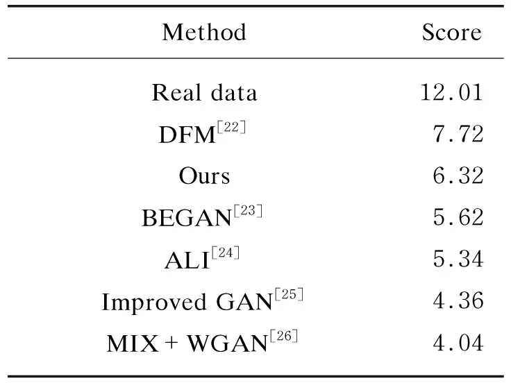
Table 1 Numerical results of IS

Figure 10 shows some intermediate results when the CIFAR-10 is used to further test our method. As the number of training increases, the generated image changes from fuzzy to sharp, and the generated image distribution is gradually closer to the real image distribution. It is noted that here we combine 64 pieces of images individually generated into one.

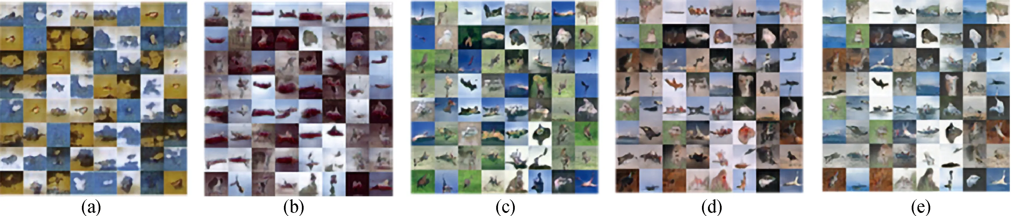
Fig. 10 Random samples generated with different training steps on CIFAR-10: (a) 20 000; (b) 40 000; (c) 60 000; (d) 80 000; (e) 100 000

5 Conclusions

An improved BEGAN with the additional skip-connection technique is proposed in this paper.An alternative time-scale update rule is adopted to balance the learning rates of the generator and the discriminator. The results of qualitative visual assessments show that high quality images can be created by the improved BEGAN when 0.5<γ<1. Furthermore, the performance of the proposed method is quantitatively evaluated by FID and IS. The FID for the proposed method and the BEGAN with CelebA dataset are 24.57 and 84.19, respectively. At this point, the performance of our method increases by 3.4 times. The other test results for CIFAR-10 dataset show that the FID is 57.96, which are also lower than 77.27 of the BEGAN. In addition, the ISs for the proposed method and the BEGAN are 6.32 and 5.62, respectively. Our method is also slightly better than the BEGAN. However, it should be pointed out that the performance of the proposed method is better than other compared methods except for the DFM. This result is predictable because the method of DFM directly aims to match the data distribution. In short, the experiment results can confirm that the use of such imbalanced learning rate updates and the skip-connection technique can improve the performances of image generation methods. In future work, we will try to add the low rank constraint to lead to generation of high quality images with lower rank.