Chao WANG （王超）， Xiu-lei FAN （范秀磊）， Pei-fang WANG （王沛芳）， Jun HOU （侯俊）， Jin QIAN （钱进）Key Laboratory of Integrated Regulation and Resource Development on Shallow Lakes， Ministry of Education，College of Environment， Hohai University， Nanjing 210098， China， E-mail: cwang@hhu.edu.cn

Flow characteristics of the wind-driven current with submerged and emergent flexible vegetations in shallow lakes*

Chao WANG （王超）， Xiu-lei FAN （范秀磊）， Pei-fang WANG （王沛芳）， Jun HOU （侯俊）， Jin QIAN （钱进）Key Laboratory of Integrated Regulation and Resource Development on Shallow Lakes， Ministry of Education，College of Environment， Hohai University， Nanjing 210098， China， E-mail: cwang@hhu.edu.cn

A pneumatic annular flume is designed to simulate the current induced by the wind acting on the water surface in shallow lakes and the experiments are conducted to investigate the influence of submerged and emergent flexible vegetations of different densities on the flow characteristics （e.g.， the flow velocity， the turbulence intensity， the vegetal drag coefficientDC and the equivalent roughness coefficientbn） at different wind speeds. Vallisneria natans （V. natans ） and Acorus calamus （A. calamus）widely distributed in Taihu Lake are selected in this study. It is indicated that the vertical distribution profiles are in logarithmiccurves. The stream-wise velocity rapidly decreases with the increasing vegetation density. The flow at the lower layer of the vegetation sees compensation current characteristics when the vegetation density is the largest. The turbulence intensity in the flume without vegetation is the highest at the free surface and it is near the canopy top for the flume with V. natans. The turbulence intensity near the bottom in the flume with vegetation is smaller than that in the flume without vegetation. A. calamus exerts much larger resistance to the flow than V. natans. The variations ofDC andbn caused by the vegetation density and the wind speed are also discussed.

velocity profile， turbulence intensity， flow resistance， aquatic vegetation， wind-driven current

Introduction

Aquatic plants， widely distributed in many rivers and lakes， are important components in aquatic ecosystems［1］. They play an important role in the flow characteristics such as the flow velocity， the turbulence intensity， the flow resistance， and also have a great potential to alter the sediment re-suspension， the contamination transportation and the geomorphology［2］. Therefore， it is important to understand the interactions between the flow and the vegetation.

The velocity profile is in an “S” shape or a reversed “S” shape in flows with a submerged vegetation and in a “J” shape for an emergent vegetation［3］. Generally， the velocity profile is grouped into two or three layers and even four layers. Li et al.［2］devided the vertical distribution of velocity in an open-channel flume with a submerged vegetation into three layers: the upper non-vegetated layer， the middle canopy layer and the lower sheath section layer. The velocity maximum value appears at the water surface and the inflection point is commonly located near the canpoy layer［2，4］. The vegetation characteristics and the configuration have a great impact on the flow turbulence intensity［5］. The turbulence intensity is the largest near the vegetation canopy top［2］and at the level of the maximum deflected vegetation height. With the increase of the vegetation density， the turbulence intensity increases at the base of the slope and decreases along the sloped bank surface within the main channel［6］.

The effects of the aquatic vegetation on the flow characteristics are primarily determined by the vegetation-induced resistance， and the studies exploring the impact of the aquatic vegetation on the flow resistance（e.g.， the drag coefficientDC， the roughness coefficient n） date back to the 1950s［2，4，7］. Generally， the drag coefficientDC indicates that the vegetation drag force is strongly a function of the Reynolds number and with a significantly positive correlation with the vegetation density［8］. However， another study［9］produced a contrary result that the value of the drag coefficient is lower with a higher vegetation density. The equivalent roughness coefficient is usually used to simulate the flow within highly resistive strips and the Manning roughness coefficient is usually applied in the ecosystem and was studied most thoroughly. The vegetation density， the diameter， the flexibility and the height are the important factors that affect the Manning coefficient. Chow［7］found that the Manning coefficient is also a function of the Reynolds number and increases with the flow water depth， which is typical for row crops partially submerged along rivers. Kouwen and Fathi-Moghadam［10］proposed a function for the roughness coefficient of the flow depth with flexible vegetations.

In the previous studies， the influences of the vegetation on the flow structure and the flow resistance were identified， most of which were discussed in the current induced by gravity in open channels. Few studies investigated the flow characteristics in shallow lakes with a dense vegetation， where the current is induced by the wind acting on the water free surface. The water in the region with a dense aquatic vegetation is usually clear. In addition， the eutrophication degree in the herbaceous type lake is also lower than that in the non-herbaceous type lake. Investigating the impact of the vegetation on the flow structure and the resistance contributes to the understanding of the mechanism of the environmental and ecological functions of aquatic vegetations in a herbaceous type lake.

In this study， a pneumatic annular flume is designed to simulate the current induced by the wind acting on the water surface in shallow lakes. The current in the flume is driven by the wind continuously generated by a blast blower. The type of the driving force in this experiment is more close to that under the natural conditions and different from some other studies［11］， in which the surface driving force is caused by a mechanical method. Hua et al.［11］used a driving device with several axially assembled dishes to drive the flow in an annular flume and investigated the vegetal flow velocity profiles. Banerjee et al.［12］used a fan to generate the wind in the flume with a length of only 2.115 m， while the flume in their experiment was annular， and the length could be considered as infinite. So， the water flow in this experiment could be developed more fully. The equipment used in this study may be more scientific to simulate the wind-driven current.

The main objective of this study is to investigate the influence of submerged and emergent flexible vegetations on the flow structure and resistance under the wind-driven current. To accurately reflect the influence of the flexible vegetation on the flow characteristics， the natural vegetations of V. natans and A. calamus， widely distributed in Taihu Lake， are planted with different densities in the pneumatic annular flume. The vertical profiles of the stream-wise velocity and the turbulence intensity in three dimensions are studied. In addition， the drag coefficient and the equivalent roughness coefficient are also investigated.

1. Materials and methods

1.1Experimental instrument and materials

The experiments are conducted in the pneumatic annular flume （of a national invention patent of China（No. 200710025671.3））. The total height of the flume is 0.95 m， and the width of the flow cross section is 0.30 m. A blast blower is used to produce a fully developed flow by the driving force of the wind acting on the water surface， and the wind is transported into the annular flume by a pipe. The opening extent of a valve could be set to simulate different levels of the true wind speed acting on the water surface in shallow lakes. A plan view of the pneumatic annular flume is shown in Fig.1. It could be assumed that the driving force induced by the wind in this study is consistent with that in the true shallow lakes. In addition， the vertical distribution of the stream-wise velocity is investigated by using this equipment， and the results also agree with those obtained in field observations in Taihu Lake［13］.

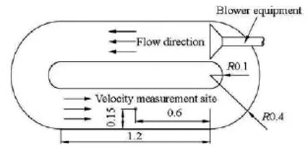
Fig.1 Plan view of the pneumatic annular flume （m）

The experiments are carried out with seven flumes， placed in greenhouse， one without vegetation，three with submerged vegetation and the other three with emergent vegetation， named as NV， SV1， SV2，SV3， EV1， EV2， and EV3， respectively. Typical submerged and emergent vegetations （for V. natans and A. calamus） are selected in this study. There are wide areas with shallow water （0.03 m-0.06 m in depth）where aquatic plants grow densely in Taihu Lake. In such regions， the density of V. natans ranges from 162 IP/m2to 387 IP/m2， and the density of A. calamus is 127 IP/m2-212 IP/m2. The general heights of V. natans and A. calamus are approximately 0.30 m-0.50 m and 0.50 m-0.80 m， respectively. The vegetation density plays an important role in the flow resistance caused by the vegetation. The vegetations are planted in the flumes with different densities， 100 IP/m2in SV1， 200 IP/m2in SV2 and 300 IP/m2in SV3，50 IP/m2， 100 IP/m2and 200 IP/m2in EV1， EV2 and EV3， respectively. Some physical properties of V. natans and A. calamus used in this experiment are as follows: the average length of the V. natans and A. calamus is 0.40 m and 0.65 m， respectively； the V. natans and A. calamus both contains 6-9 groups of foliage per plant， which grow directly from the root，and the mean width of the foliage is approximately 0.008 m and 0.012 m， respectively. The frontal area per canopy volume called the canopy density reflects the characteristics of the blockage provided by the canopy. The canopy density varies in the vertical direction［14］， and is calculated as

where n is the vegetation density， Afis the average frontal area of ten randomly selected plants， estimated at 0.01 m intervals in the vertical direction by tracing the plant silhouettes onto the grid paper， and Δz= 0.01 m. The canopy densities of V. natans and A. calamus are calculated when n =100IP/m2in this study， and the profile of a（z） is shown in Fig.2.

Fig.2 Profile of canopy density for V. natans and A. calamus varied with vegetation height （HV）， when the vegetation density is 100 IP/m2

The main active layer participating in the dynamic exchange between the overlying water and the sediments is the 0.05 m-0.10 m of sediments in the surface of the shallow lake. In addition， taking into account the growth requirements of the vegetation， the thickness of the experimental sediments is designed as 0.15 m. The sediment samples are collected from East Taihu Lake （N31o08′24″， E120o50′39″） which is a typical herbaceous type shallow lake. The water area of East Taihu Lake is 131 km2with an average water depth of 1.20 m. The wet bulk density of sediments in this region is 1.23×103kg/m3to 1.52×103kg/m3with the average value of 1.40×103kg/m3. The pH value of the sediments is in the range of 6.83-7.24 with an average of 7.12. The experimental water is just the tap water from laboratory and is injected into the flume slowly via a siphon until the water depth is 0.50 m. The 0.50 m depth of water is within the scope of the general water depth in the shallow region in Taihu Lake with a lush vegetation. The side view of the flume planted vegetation is shown in Fig.3. The flume is placed in the greenhouse for 20 d to simulate the field conditions after the vegetation is planted， then the experiments starts.

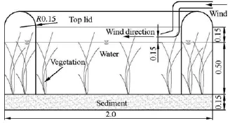
Fig.3 Side view of the pneumatic annular flume （m）

1.2Experiment conditions and flow measurements

According to the study of You et al.［15］， three different wind speeds are implemented in the flumes to simulate the small wind （2.0 m/s-4.0 m/s）， the medium wind （5.0 m/s-7.0 m/s）， and the strong wind（＞8.0m/s） in Taihu Lake， respectively. The experimental wind speeds are approximately 3.0 m/s， 6.0 m/s and 9.0 m/s， as measured with a thermal anemometer，and they are numbered as conditions 1-3.

After each condition is kept for 8 h， the flow structure becomes stable， the velocity measurement starts. The measurement is made at 0.01 m intervals from the bottom to 0.10 m near the bed and then at 0.025 m intervals from 0.10 m to 0.50 m towards the free water surface. The velocity measurement site （black dot） is shown in Fig.1. A three-dimensional sideway 16 MHz macro-acoustic doppler velocimetry （MacroADV）（SonTek， San Diego， CA， USA） is utilized to measurethe instantaneous velocity and the turbulence along the vertical direction at a frequency of 10 Hz with the sampling time of 30 s. Therefore， a total of 300 data are acquired to calculate the average velocity and the turbulence values for each measurement point with a post-processing software， WinADV［16］.

Table 1 Experimental results

1.3Drag coefficientDC and equivalent roughness coefficientbn

To further explore the behavior of the vegetation in the wind-driven current， the vegetal drag coefficient CDand the equivalent roughness coefficient nbare calculated in this study. The the drag coefficient in a wind- driven current is expressed as［11］

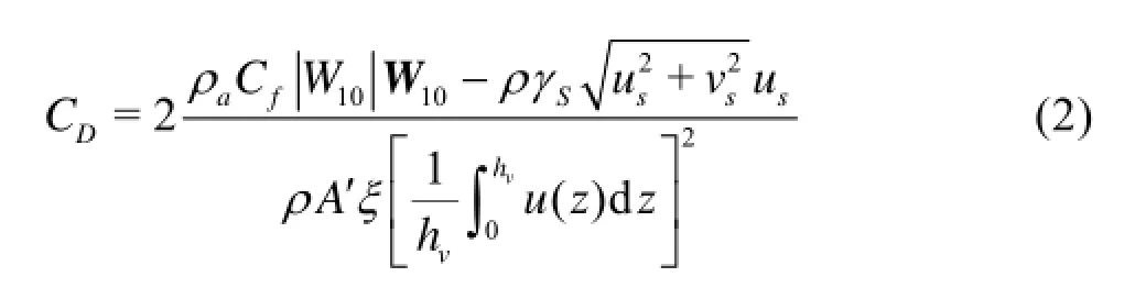
where DC is the drag coefficient， and assumes a same value for each individual plant，aρ is the air density， W10is the velocity of the wind at a level 10 m over the lake surface， fC and sγ are the drag coefficients of the water surface and the bottom， ρ is the water density，su andsv are the velocities of the water bottom in the stream-wise and lateral directions， respectively. A＇ is the projected area in the stream-wise direction of each vegetation， ξ is the vegetation density，vh is the vegetation effective height， and u is the velocity around the vegetation， related to the water depth.

The equivalent roughness coefficientbn can be calculated as follows［11］

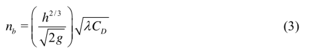
where h is the flow depth， g and λ are the acceleration of gravity and the vegetal area coefficient， respectively.

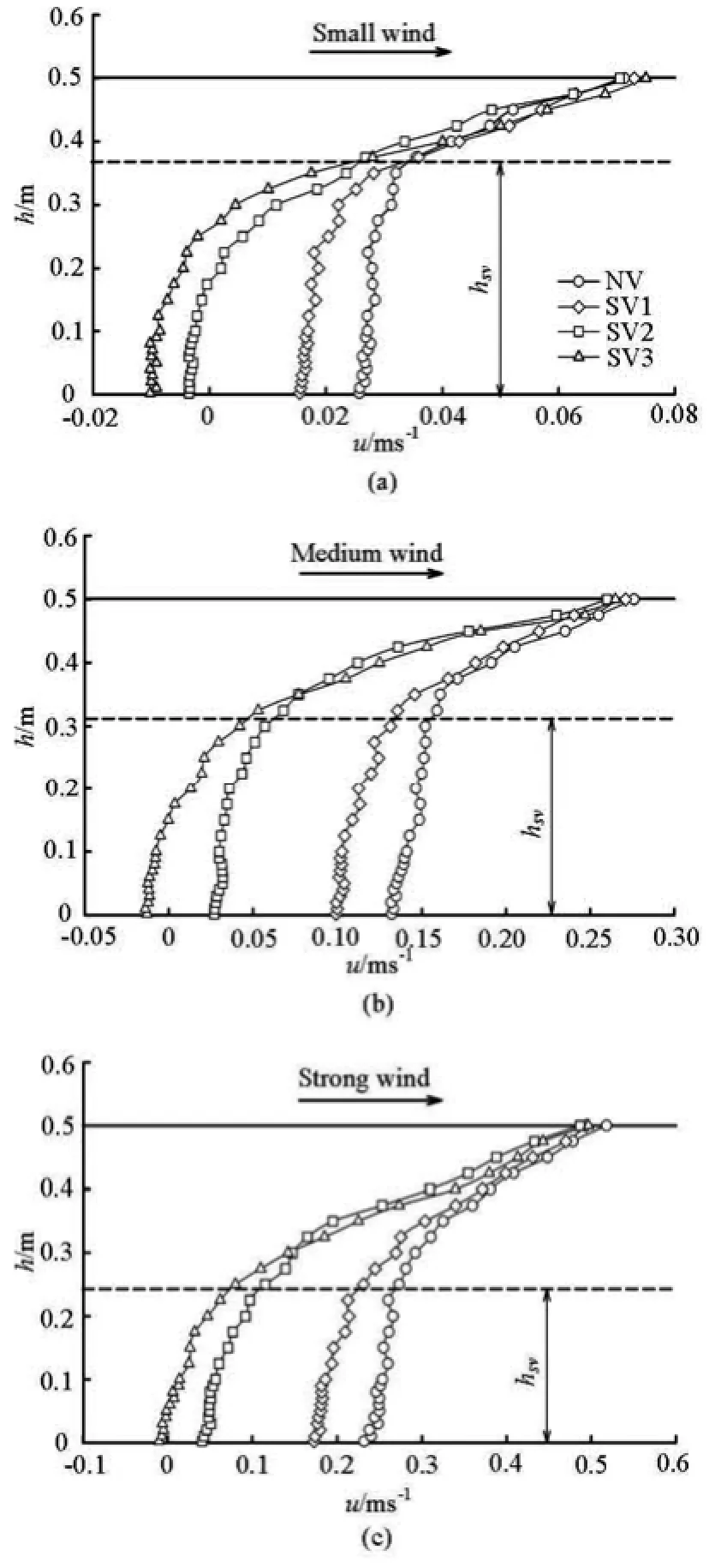
Fig.4 Vertical distribution profiles of stream-wise velocity at different wind speeds in flumes SV1， SV2 and SV3. Here h represents the water depth， u represents the stream-wise velocity andsvh represents the average effective height of V.natans in the three flumes

Fig.5 Vertical distribution profiles of stream-wise velocity at different wind speeds in flumes EV1， EV2 and EV3. Hereevh represents the average effective height of A. calamus in the three flumes

2. Results

2.1Velocity profiles

As shown in Fig.4 and Fig.5， the relationship between the stream-wise velocity and the water depth（the distance between the velocity measurement site and the sediment surface） could be described by a logarithmic-curve in the flume NV. The maximum velocity appears at the water surface and decreases towards the water bottom. The stream-wise velocity increases with the increasing wind speed. The mean stream-wise velocity increases by about 3.82 times when the wind speed increases from small to medium levels （Table 1）. The stream-wise velocity gradient near the free surface is significantly larger than that in the middle and bottom parts of the water. As shown in Table 1， the effective height of the vegetation decreases with the increasing wind speed， especially for the submerged vegetation. The variation of the effective height for the emergent vegetation is negligible. The emergent vegetation exerts a greater resistance to theflow than the submerged vegetation. The mean stream-wise velocities are 0.1338 m/s and 0.0501 m/s in the flumes SV1 and EV22（in which the vegetation densities are both 100 IP/m） under the condition of a medium wind， while the mean stream-wise velocity is 0.1599 m/s in the flume NV （Table 1）. As shown in Fig.4 and Fig.5， the vertical distribution profiles of the stream-wise velocity see significant differences， especially in the upper layer of the flume. The phenomena indicate that the type of vegetations does play an important role in altering the flow characteristics in the flume.

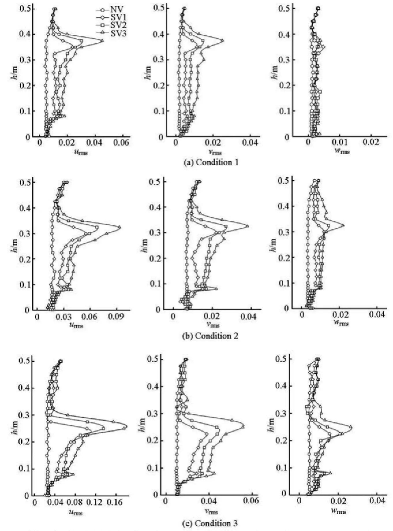
Fig.6 Vertical distributions of turbulence intensityrmsu，rmsv andrmsw （m/s） at different wind speeds in flumes SV1， SV2 and SV3. Here the horizontal dotted line represents the average effective height of V. natans in the three flumes

As shown in Fig.4， the vertical distribution profiles of the stream-wise velocity in the flumes SV1，SV2 and SV3， could be roughly divided into two layers: the non-vegetation layer （from the vegetation canopy top to the water surface） and the vegetation layer （within the effective height of the submerged vegetation）. The stream-wise velocity in the non-vegetation layer is much larger than that in the vegetation layer. The size of the vegetation layer decreases with the increasing wind speed. The height of the layer decreases from approximately 0.37 m to 0.24 m when the wind increases from small level to strong level， for example. In the non-vegetation layer， the stream-wise velocity profile is similar to that in the flume NV， also following a logarithmic law. The stream-wise velocity increases with the increasing vegetation densities except for the case of 100 IP/m2. The maximum velocity occurs at the water surface and its value is veryclose to that in the flume NV. In the vegetation layer，the stream-wise velocity is greatly reduced because of the presence of the submerged vegetation and sees a decreasing trend as the water depth increases. In addition， the stream-wise velocity increases with the increasing wind speed. The maximum and minimum stream-wise velocities appear at the submerged vegetation canopy top and the bottom， respectively. Under the condition of a strong wind， V.natans is dominantly affected by the current， the leaves are close to the flume bottom. Then the stream-wise velocity decreases significantly because the resistance near the bottom increases greatly. Meanwhile， the negative velocity appears in the lower part of the vegetation layer only when the submerged vegetation density is 300 IP/m2and the negative velocity region size is further reduced in the medium and strong winds. For all submerged vegetation densities， the stream-wise velocity is much smaller than that in the flume without vegetation and is reduced greatly as the submerged vegetation density increases.

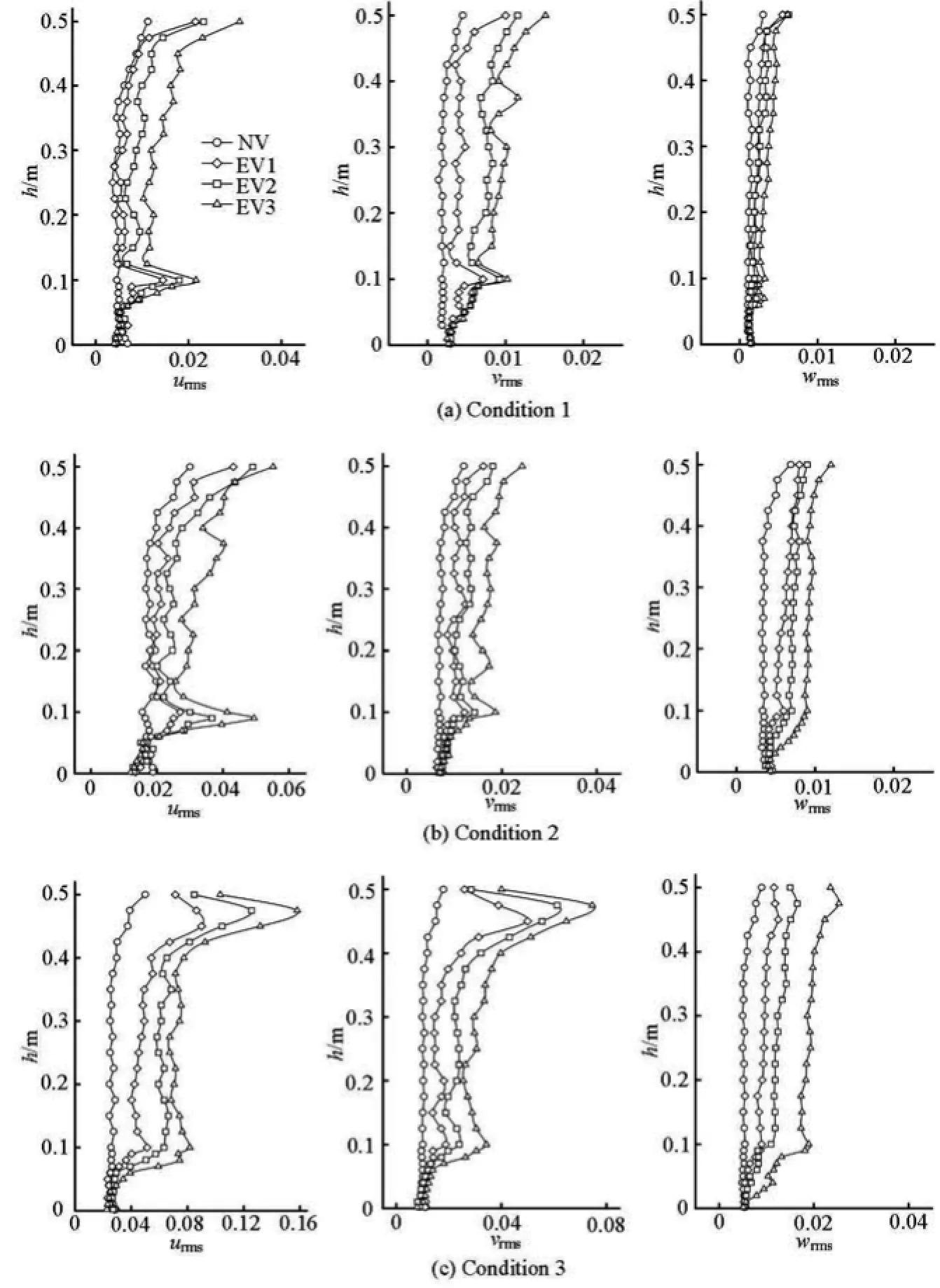
Fig.7 Vertical distributions of turbulence intensityrmsu，rmsv andrmsw （m/s） at different wind speeds in flumes EV1， EV2 and EV3. Here the horizontal dotted line represents the average effective height of A. calamus in the three flumes

As shown in Fig.5， only the vegetation layer appears in the flume with A. calamus， and the nonvegetation layer in the flume EV3 could be ignored. The stream-wise velocity sees a decreasing trend with the increasing wind speed. As shown in Table 1， the average stream-wise velocity increases from 0.0262 m/s to 0.2239 m/s when the wind increases from small to strong levels in the flume EV1， for example. Under a strong wind， the top of A. calamusis submerged， and the velocity at the water surface increases significantly owing to the direct action of the wind driving force. The maximum and minimum values occur at the water surface and the bottom， respectively. And， the maximum value is much smaller than that in the flume NV. Meanwhile， the negative velocity appears in the lower part of the emergent vegetation when the wind is in medium and strong levels in the flume EV3. In addition， with the increase of the emergent vegetation density， the stream-wise velocity is greatly reduced， for example， the mean stream-wise velocity decreases by about 60%， when the vegetation density increases from 50 IP/m2to 100 IP/m2（Table 1） under a medium wind， indicating that the vegetation density plays a vital role in altering the vegetation flow resistance in the flume.

Table 2 The Drag coefficientDC and the equivalent roughness coefficientbn of V. natans and A. calamus with different densities at different wind speeds

2.2Turbulent intensity

To investigate the influence of the submerged and emergent vegetations on the turbulence intensity in the current induced by the wind acting on the water surface， the turbulence intensitiesrmsu，rmsv andrmsw（in the stream-wise， span-wise and vertical directions，respectively） at different wind speeds are measured（Fig.6 and Fig.7）. As shown in Fig.6，rmsu，rmsv and wrmsin the flume NV see similar trends and the maximum values appear at the free surface. The turbulence intensities decrease slightly with the water depth and increase near the flume bed. In the flume with a submerged vegetation， the peaks ofrmsu，rmsv andrmsw appear around the plant canopy top and the stem base at a height of 0.06 m-0.09 m. In general， the turbulence intensity profiles above the plant canopy top are similar to those in the flume without vegetation， and the turbulence intensities between the plant canopy and the plant stem base are stable with a nearly constant value. The turbulence intensities near the flume bottom are unstable and weak， and their values are even smaller than that in the flume NV. The turbulence intensities near the plant canopy rapidly vary for large vegetation densities and vary gently for small vegetation densities. In addition， the value of the turbulence intensity increases rapidly with the increasing wind speed.

As shown in Fig.7， in the flume with the emergent vegetation， the turbulence intensity profiles under the condition of small and medium wind levels are different from those under the condition of a strong wind. When the wind speed is in small and medium levels， the peaks ofrmsu，rmsv andrmsw are located at the plant stem base at a height of 0.09 m-0.11 m. Below the plant stem base， the turbulence intensities are unstable and even smaller than those in the flume without vegetation. The turbulence intensities increase slightly upwards the free surface from the plant stem base and the maximum value occurs at the free surface. The values of the turbulence intensities above the plant stem base are almost stable for all vegetation densities. The turbulence intensities also increase with the vegetation density at the three wind speeds. Under the condition of a strong wind， A. calamus canopy top is dominantly affected by the current. Thus， the maximum turbulence intensity occurs around the canopy top again and its location is gently migrated upwards with the increase of the vegetation density.

2.3Drag coefficient and equivalent roughness coefficient

The values ofDC andbn of V. natans and A. calamus are obtained by Eq.（2） and Eq.（3） and are listed in Table 2. Obviously， due the variation of the wind speed and the vegetation density， the changes of CDand nbof V. natans are similar to those of A. calamus （Table 2）. As shown in Table 2， CDand nbincrease with the vegetation density for both submerged and emergent vegetations. However， the increase of the wind speed reduces the values of CDand nb. Meanwhile， the values of CDand nbof the submerged vegetation are much smaller than those ofthe emergent vegetation， for instance， at a small level of the wind theDC takes a value of 200 IP/m2for V. natans， even smaller than 100 IP/m2for A. calamus.

3. Disscussions

3.1Velocity profiles

The vertical distribution profiles of the streamwise velocity in the flume NV follow a logarithmic law and similar results were obtained in experimental studies and field observations in Taihu Lake［11，13］. The profile of the stream-wise velocity in the flume with submerged and emergent vegetations generally also follows the logarithmic law. The stream-wise velocity profile in a flexible vegetated current driven by the wind stress in this study is greatly different from the typical velocity profile in the open channel caused by the gravity drive. The typical velocity profile takes an“S” shape or a reversed “S” shape in the flow with submerged vegetations and a “J” shape in the flow with emergent vegetations. The difference is due to the entirely dissimilar current driving force. The negative velocity appears in the lower part of the vegetation only when the vegetation density is the largest in this study， and its region size decreases with the increasing wind speed. The phenomenon could be explained as follows: because the current driving force is the wind acting on the water surface in this experiment， the transmission of the water momentum is from the water surface to the bottom. The momentum is transferred to a deep water by the viscosity， which consumes energy due to the resistance exerted by the vegetation to the flow. As the resistance increases with the vegetation density， it will be large enough to cause the water momentum exhausted in the upper layer and could not reach the lower layer when the vegetation density is the largest as in this study. Due to the energy conservation， the flow velocity in the water bottom has to be reduced and even changes the direction， reflecting the compensation current characteristics. As the wind speed increases， the bending deformation of the vegetation becomes larger， and then the drag force exerted by the vegetation to the current is reduced. In addition， the momentum could be transferred closer to the bottom because more kinetic energy is obtained from the stronger wind. Thus， the region size of the negative velocity is decreased. As stated previously， the occurrence of the compensation current is mainly due to the driving force on the water surface， moreover， the wind speed and the vegetation density are also the significant influential factors.

The morphology of V. natans and A. calamus in this experiment is different from that in the previous studies［2，4］， in which the artificial plant with a certain length of obvious stem is usually used. V. natans and A. calamus both contain basal leaves which directly grow from the root. And the canopy density increases gently from the plant root to the stem base， then to the foliage （Fig.2）. Therefore， the inflection point of the stream-wise velocity does not appear obviously in the bottom region of the vegetation， and the velocity profile in the flume with V. natans is divided into two layers， and one layer with A. calamus. The streamwise velocity profile for the lower vegetation layer in the flume with V. natans is similar with that in the flume with A. calamus. The canopy densities of V. natans and A. calamus both decrease with the increasing water depth （Figs.1， 3）， which increases the velocity gradient in the upper region of the vegetation as compared with that in the lower region. The large canopy density with a small vegetation space in the stream-wise direction greatly reduces the stream-wise velocity， thus the velocity is significantly reduced （i.e.，with a large velocity gradient）. The stream-wise velocities in the flume with V. natans and A. calamus are both much smaller than that in the flume without vegetation， especially for A. calamus which features smaller flexibility， wider leaves and larger water-resisting area. Meanwhile， the drag force exerted by A. calamus leaves above the water surface for the wind might be another reason for a greater resistance than V. natans in this study. A large shear flow appears in the upper non-vegetation layer due to the presence of a submerged vegetation. For a large vegetation density （200 IP/m2， 300 IP/m2in this study）， the stream-wise velocity over the canopy top increases because the dense leaves of V. natans force up more flow from the lower vegetation layer to the upper nonvegetation layer.

3.2Turbulence intensity

The wind kinetic energy is converted into the flow kinetic energy due to the work done by the driving force of the wind acting on the water surface. Therefore， the momentum exchanges most fiercely（the maximum turbulence intensity） near the free surface in the flume without vegetation， which is different from that in the previous studies［2］. Moreover， the turbulence intensity is larger at the free surface due to the obstruction of the emergent vegetation to the flow. The flow turbulence intensity largely fluctuates in the flume with vegetation， and the turbulence intensity profile with a submerged vegetation is distinctly different from that with an emergent vegetation， indicating that the vegetation type plays an important role in the turbulence characteristics.

The turbulence intensity is the largest near the canopy top in the flumes with submerged and emergent vegetations under a strong wind， suggesting that the fluctuation of the uneven flow is most fierce near the canopy top region. The phenomenon could be explained as follows: the flow kinetic energy is converted into the turbulent kinetic energy by the aquatic plantsbecause the foliage sways near the vegetation canopy top. Meanwhile， the turbulence is caused by the vortices resulting from the flow instability and the largest shear at the flow-vegetation interface occurs near the vegetation canopy top. The Kelvin-Helmholtz （K-H）instability， occurred near the vegetation canopy top，generates large numbers of continuous vortices controlling the momentum exchange. The momentum exchange mostly appears at the interface between the upper region without vegetation and the vegetation canopy top layer， thus the vegetation absorbs a large momentum from the current near the canopy top and transfers a part of the momentum into the vegetation bottom. The instability of the flow is increased at the vegetation stem base because the stem base is rigid and the canopy is dense there. Therefore， at the vegetation stem base some flow kinetic energy is converted into the turbulent kinetic energy again and the peak turbulence intensity is reached. The vegetation stem base consumes the flow kinetic energy and apparently inhibits the turbulence transferred from the vegetation canopy. Meanwhile， the turbulence intensity decreases rapidly below the stem base and is even smaller than that in the flume NV. The energy flow path in this study， from the water free surface to the bottom， might be the reason that can explain this phenomenon.

In addition， the turbulence intensity below the stem base is also unstable because of the bottom boundary at the flume bed. The large vegetation density with dense leaves leads to a large shear at the flowvegetation interface， especially near the canopy top. Thus， the turbulence intensity increases with the vegetation density. Similar results were also found in the previous studies［2，17，18］. The maximum turbulence intensity location is migrated upwards with the increase of the vegetation density resulting from increase of the effective height of the vegetation （Table 1）. The canopy dense leaves increase the flow velocity and the instability above the canopy top. The flow instability increases at a strong wind speed to cause a fast flow velocity with a large inertia. Thus the vegetation fiercely sways， and the turbulence vortices are quickly generated near the interface of the flow and the vegetation. Meanwhile， the height of the canopy top decreases because the vegetation leaves are dominantly affected with a large deflection angle by the fast flow，especially for V. natans. Therefore， with an increasing wind speed， the value of the turbulence intensity increases and the maximum value location is migrated downwards.

3.3Flow resistance

The stream-wise velocity increases rapidly with the increasing wind speed （Table 1）. The effective height of the vegetation decreases because the leaves of V. natans and A. calamus are dominantly affected by the rapid current. Therefore， the resistance to the flow exerted by the vegetation becomes weak， with the decrease ofDC andbn. Wang et al.［19］also found that the effective height of the vegetation decreases with the flow velocity and a larger effective height would cause a greater flow resistance. The effect of the flexible vegetation is equivalent to that of a rough bed when the deflection angle increases to a certain magnitude. As the current velocity increases to a certain level， the drag coefficient and the equivalent roughness coefficient would decrease to a constant［11］. The Reynolds numbers increases with the wind speed（Table 1）， thusDC andbn also decrease with the increasing Reynolds numbers. Similar findings were also reported in the previous studies［11，20］.

The vegetation density is a vital factor controlling the vegetation flow resistance［2，9］. As shown in Table 2， the values of the drag coefficient and the equivalent roughness coefficient increase with the vegetation density， suggesting that the large vegetation density could cause a high flow resistance in the flume. The dense leaves for a large vegetation density intensifies anisotropy. The flow directions around leaves and stems vary because of the different morphologies and orientations of the leaf surface， hence the flow resistance increases［2］. The resistance to the flow exerted by A. calamus is much stronger than that by V. natans. The weak reconfiguration ability of the emergent vegetation with rigid relative leaves might increase the flow resistance， and the high free flow depth of the submerged vegetation might decrease the resistance to the flow. Moreover， the wider leaves of A. calamus might be another factor for its greater resistance than that of V. natans.

4. Conclusions

（1） The vertical distribution profile of the streamwise velocity is in a logarithmic-curve. A compensation current appears at the lower layer of the vegetation under the condition of the largest vegetation density （200 IP/m2for A. calamus and 300 IP/m2for V. natans in this study）， and the wind speed decreases the height of the compensation current. The vertical distribution profile of the stream-wise velocity is divided into two layers for V. natans， the non-vegetation layer and the vegetation layer. While only the vegetation layer appears in the flume with A. calamus. Moreover， the stream-wise velocity rapidly decreases with the increasing vegetation density.

（2） The value of turbulence intensity in the flume NV and the flume with A. calamus is the highest at the free surface because of the driving force directly exerted on the water surface. The turbulence intensity in the flume with V. natans is the largest near the canopy top because the foliage prominently sways there. Thepeak turbulence intensities of V. natans and A. calamus both occur near the rigid stem base. The value of the turbulence intensity increases with the vegetation density and the wind speed. The turbulence intensity near the bottom in the flume with vegetation is even smaller than that in the flume without vegetation，suggesting that the vegetation might play a significant role in the re-suspension process of the sediments and the aquatic environment in shallow lakes.

（3） A. calamus shows a much larger resisting ability to the current than V. natans. The increase of the wind speed decreases the drag coefficient and the equivalent roughness coefficient， indicating that the strong wind could decrease the vegetal resistance to the current. The flow resistance increases with the vegetation density， suggesting that the vegetation density plays a vital role in the vegetation flow resistance.

References

［1］WANG Chao， ZHENG Sha-sha and WANG Pei-fang et al. Interactions between vegetation， water flow and sediment transport: A review［J］. Journal of Hydrodynamics， 2015，27（1）: 24-37.

［2］LI Y.， WANG Y. and ANIM D. O. et al. Flow characteristics in different densities of submerged flexible vegetation from an open-channel flume study of artificial plants［J］. Geomorphology， 2014， 204: 314-324.

［3］GHISALBERTI M.， NEPF H. M. The limited growth of vegetated shear layers［J］. Water Resources Research，2004， 40（7）: 1-12.

［4］WANG Chao， ZHANG Wei-min and WANG Pei-fang et al. Effect of submerged vegetation on the flowing structure and the sediment resuspension under different windwave movement conditions［J］. Journal of Safety and Environment， 2014， 14（2）: 107-111（in Chinese）.

［5］JALONEN J.， JÄRVELÄ J. Estimation of drag forces caused by natural woody vegetation of different scales［J］. Journal of Hydrodynamics， 2014， 26（4）: 608-623.

［6］CZARNOMSKI N. M.， TULLOS D. D. and THOMAS R. E. et al. Effects of vegetation canopy density and bank angle on near-bank patterns of turbulence and Reynolds stresses［J］. Journal of Hydraulic Engineering， ASCE，2012， 138（11）: 974-978.

［7］CHOW V. T. Open-channel hydraulics［M］. New York，USA: McGraw-Hill， 1959.

［8］KOTHYARI U. C.， HAYASHI K. and HASHIMOTO H. Drag coefficient of unsubmerged rigid vegetation stems in open channel flows［J］. Journal of Hydraulic Research，2009， 47（6）: 691-699.

［9］CHIEW Y. M.， TAN S. K. Frictional resistance of overland flow on tropical turfed slope［J］. Journal of Hydraulic Engineering， ASCE， 1992， 118（1）: 92-97.

［10］ KOUWEN N.， FATHI-MOGHADAM M. Friction factors for coniferous trees along rivers［J］. Journal of Hydraulic Engineering， ASCE， 2000， 126（10）: 732-740.

［11］ HUA Z. L.， WU D. and KANG B. B. et al. Flow resistance and velocity structure in shallow lakes with flexible vegetation under surface shear action［J］. Journal of Hydraulic Engineering， ASCE， 2013， 139（6）: 612-620.

［12］ BANERJEE T.， MUSTE M. and KATUL G. Flume experiments on wind induced flow in static water bodies in the presence of protruding vegetation［J］. Advances in Water Resources， 2015， 76: 11-28.

［13］ QIAN Jin， ZHENG Sha-sha and WANG Pei-fang et al. Experimental study on sediment resuspension in Taihu Lake under different hydrodynamic disturbances［J］. Journal of Hydrodynamics， 2011， 23（6）: 826-833.

［14］ NEPF H. M.， VIVONI E. R. Flow structure in depthlimited， vegetated flow［J］. Journal of Geophysical Research： Oceans， 2000， 105（C12）: 28547-28557.

［15］ YOU Ben-sheng， ZHONG Ji-cheng and FAN Cheng-xin et al. Effects of hydrodynamics processes on phosphorus fluxes from sediment in large， shallow Taihu Lake［J］. Journal of Environmental Sciences， 2007， 19（9）: 1055-1060.

［16］ WAHL T. L. Analyzing ADV data using WinADV［C］. Procceedings of the Joint Conference on Water Resources Engineering and Water Resources Planning and Management. Reston， Virginia， USA， 2000.

［17］ NEZU I.， ONITSUKA K. Turbulent structures in partly vegetated open-channel flows with LDA and PIV measurements［J］. Journal of Hydraulic Research， 2001， 39（6）: 629-642.

［18］ STOESSER T.， SALVADOR G. P. and RODI W. et al. Large eddy simulation of turbulent flow through submerged vegetation［J］. Transport in Porous Media， 2009，78（3）: 347-365.

［19］ WANG Pei-fang， WANG Chao and ZHU David Z. Hydraulic resistance of submerged vegetation related to effective height［J］. Journal of Hydrodynamics， 2010， 22（2）: 265-273.

［20］ TSIHRINTZIS V. A. Discussion of “variation of roughness coefficients for unsubmerged and submerged vegetation”［J］. Journal of Hydraulic Engineering， ASCE，2001， 127（3）: 241-244.

（May 19， 2015， Revised July 1， 2016）

* Project supported by the National Science Funds for Creative Research Groups of China （Grant No. 51421006）， the Program for Changjiang Scholars and Innovative Research Team in University （Grant No. IRT13061）， the National Science Fund for Distinguished Young Scholars （Grant No. 51225901）， the Key Program of National Natural Science Foundation of China （Grant No. 41430751）， the National Natural Science Foundation of China （Grant No. 51479065） and PAPD.

Biography： Chao WANG （1958-）， Male， Ph. D.， Professor

Pei-fang WANG，

E-mail: pfwang2005@hhu.edu.cn