Xiang-bin LI （李向宾）， Nan LI （李楠）， Guo-yu WANG （王国玉）， Min-di ZHANG （张敏弟）

1. School of Nuclear Science and Engineering， Beijing Key Laboratory of Passive Safety Technology for Nuclear Energy， North China Electric Power University， Beijing 102206， China， E-mail: lixiangbin@ncepu.edu.cn

2. School of Mechanics and Vehicle Engineering， Beijing Institute of Technology， Beijing 100081， China

Reverse motion characteristics of water-vapor mixture in supercavitating flow around a hydrofoil*

Xiang-bin LI （李向宾）1， Nan LI （李楠）1， Guo-yu WANG （王国玉）2， Min-di ZHANG （张敏弟）2

1. School of Nuclear Science and Engineering， Beijing Key Laboratory of Passive Safety Technology for Nuclear Energy， North China Electric Power University， Beijing 102206， China， E-mail: lixiangbin@ncepu.edu.cn

2. School of Mechanics and Vehicle Engineering， Beijing Institute of Technology， Beijing 100081， China

The supercavitation has attracted a growing interest because of its potential for high-speed vehicle maneuvering and drag reduction. To better understand the reverse flow characteristics of a water-vapor mixture in supercavitating flows around a hydrofoil，a numerical simulation is conducted using a unified supercavitation model， which combines a modified RNG -kε turbulence model and a cavitation one. By comparing the related experimental results， the reverse motion of the water-vapor mixture is found in the cavitation area in all supercavitation stages. The inverse pressure gradient leads to reverse pressure fluctuations in the cavity，followed by the reverse motion of the water-vapor two-phase interface. Compared with the water-vapor mixture area at the back of the cavity， the pressure in the vapor area is inversely and slowly reduced，a higher-pressure gradient occurs near the cavity boundary.

supercavitation， water-vapor interface， reverse motion， pressure distribution， numerical simulation

Introduction

The cavitation flows are very complicated because of the large density variations in the flow field， the frequent pressure fluctuations， and the violent watervapor interface mass transfer［1］. They can be divided into four stages based on the special cavitation number: the inception cavitation， the sheet cavitation， the cloud cavitation， and the supercavitation. As a fully developed pattern， the supercavitation comes into being when the cavity covers the entire hydrofoil suction surface and gradually extends downstream［2］. The pressure inside a supercavitation area is often very low， where a relatively stable cavity forms. Thus， a free-stream method based on the potential flow theory was developed to predict the supercavitation dynamics， providing a linear and slender-body theory for two-dimensional supercavitating flows. However， in this method， it is assumed that the pressure distribution in a supercavitation area is uniform and equal to the local vaporization pressure， and that the cavity interface is streamlined and smooth.

In recent years， the supercavitation has attracted growing interests because of its potential for highspeed vehicle maneuvering and drag reduction［3-8］. Since 2000， numerous advanced measurement methods， equipment， and computation technologies were adopted to study supercavitating flows. Wosnik et al.［9］measured the ventilated supercavitation in turbulent bubbly wakes with a high speed camera and the particle image velocimetry， Shafaghat et al.［10］used a socalled “non-dominated sorting genetic algorithm” to carry out the shape optimization of two-dimensional cavitators in supercavitating flows， Rashidi et al. studied the ventilated supercavitation by using two methods: the VOF method and the Young's algorithm［11］. As for natural supercavitating flows around a hydrofoil， Wang et al.［2］observed that the water and vapor bubbles filled the cavitation region in the supercavitation stage. Further investigations indicate that the supercavitating flows are identified in the following three features: （1） the fluctuation cavity with periodic vortex shedding， （2） the vapor and watervapor mixture coexisting inside the cavity with a tur-bulent wake， and （3） a cavity largely filled with vapor having a two-phase tail and distinct phase boundaries in the wake region. Substantial unsteady features exist although the cavity boundary is visually smooth and the water-vapor mixture moves reversely over time［12］. In addition， the velocity in the supercavitating region has a special distribution even in the core of the cavitation region， and the lower velocity area is reduced as the cavitation number decreases.

To further understand the reverse motion mechanism of the water-vapor mixture in supercavitating flows around a hydrofoil， numerical simulations are carried out in this study， focusing on the unsteady characteristics， including the transient cavitation structures and the pressure distribution. The commercial software CFX is selected and the computational model is based on a unified supercavitation one， which combines a modified RNG -kε turbulence model and a cavitation one.

Fig.1 Schematic diagram of the hydrofoil

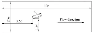
Fig.2 Sketch of the foil position in the test section

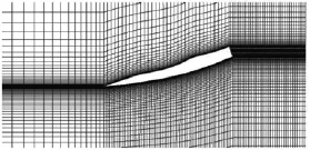
Fig.3 Grid distribution around the foil

1. Supercavitation model

1.1Hydrofoil, grid, boundary and initial conditions

A supercavitation hydrofoil investigated by Tulin［13］， as shown in Fig.1， is adopted in the present study. Figure 2 gives the hydrofoil position in the test section， of 10c in length， 2.7c in height， and 1c in width （where c is the chord length of the hydrofoil， more details can be found in Ref.［12］）. A two-dimenonal computational domain is chosen to correctly follow the geometry of the test section. An orthogonal mesh with 62 720 cells is generated as shown in Fig.3. Alternative mesh systems， with 41 540 and 85 580 cells， are also chosen to evaluate the mesh convergence of the computation. To ensure more accurate results， a finer mesh is used around the hydrofoil and the cavitation region as the related experiments indicate. The corresponding evaluation was carried out in the Ref.［14］， and the results show that a similar pressure distribution is obtained under three kinds of mesh conditions. With both accuracy and economy in mind， the mesh of medium size， 62 720 cells， is selected for the following simulation.

In this study， the foil lift angle θ is fixed at o 15，the reference velocity U is fixed at 10 m/s， the Reynolds number and the cavitation number are defined as follows:

where ν is the kinematic viscosity of the liquid，vp represents the Phase-change threshold pressure of the vapor， p∞is the reference static pressure， andlρ is the density of the liquid.

In addition， the numerical simulation conditions are as follows: the inflow velocity， the volume fractions and the turbulence quantities are specified at the inlet boundary， and the cross-sectional-averaged static pressure is imposed as the reference pressure at the outlet. A no-slip boundary condition is used at both the upper and lower walls， and the no-slip wall condition with a wall function is provided at the foil surface.

1.2Governing equations

A unified supercavitation model is based on the governing equations of both a turbulence model and a mass transport one. First， based on the Favre average form of the mass conservation equation and the Navier-Stokes equation for the momentum conservation， the RNG -kε turbulence model is as follows:

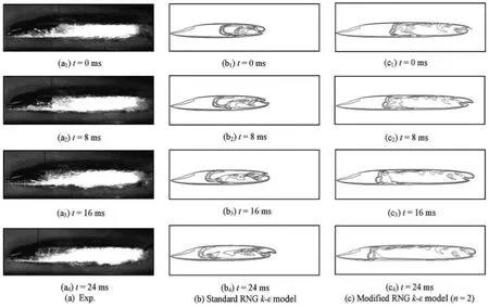
Fig.4 Instantaneous cavity structures of experiments and CFD simulations

where ρ is the density of the liquid-vapor mixture， k is the turbulent kinetic energy， ε is the turbulent dissipation rate， u is the velocity component，kp is the source term representing the production of k， the empirical constants σk=σε=0.7179， Cε1=0.085， Cε2=1.680， μ and μtrepresent the laminar viscosity and the turbulent viscosity， respectively. The turbulent viscosity is defined as follows

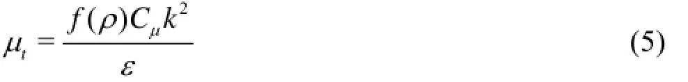
where the empirical constant Cμ=0.09. It is found that the standard RNG -kε model will result in shorter cavity lengths as compared with previously reported experimental data［15］. Accordingly， a modified RNG -kε turbulence closure model is adopted in this study. Instead of （）=fρρ in the original model，the function is defined as follows

wherevρ is the density of the liquid and the vapor，vα is the vapor volume fraction， and n is the empirical constant. The effect of the vapor phase is added.

Secondly， considering that the cavitation process is dominated by the thermodynamics and the kinetics of the phase-change dynamics in the flow field， a mass transport model （i.e.， the cavitation model） is provided based on the vapor volume fraction， just as shown in Eq.（7）. The source terms m˙+and m˙-represent the evaporation and the condensation of the phases， respectively［16］.

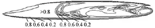
Fig.5 Instantaneous distribution of vapor volume fraction

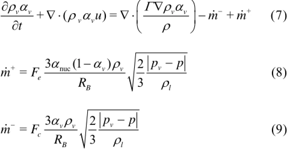
Here， Γ is the diffusion coefficient， the empirical constants=5×10-4， F=50 and F=0.01， thee c vapor bubble radius RB=10-6m ， p is the pressure in the vapor bubble. Several experimental studies have shown the significant effect of turbulence on cavitating flows. The local turbulent pressure fluctuationshould be considered in the definition of the vapor pressure， thus a modified model is adopted as follows:

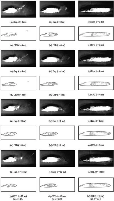
Fig.6 Instantaneous flow visualization of experiments and CFD simulations

whereturbp is the local turbulent fluctuating pressure andsatp is the saturated vapor pressure. This approach is simple and yields better outcomes［17］.

The abovementioned modifications on the turbulence and cavitation models are added into CFX software by means of self-programming. Based on the unified supercavitation model， the standard RNG -kε model and the modified one are used to simulate and compare the data with the experimental ones. Just as shown in Fig.4， the cavity length simulated by the modified model （with =2n） agrees well with the experimental one. So， the empirical constant n is selected as =2n［18］.

2. Results and discussions

Based on the above numerical model， some typical supercavitating flows around a hydrofoil are simulated in different supercavitation stages. The detailed flow structures and the pressure distribution， especially the reverse motion mechanism， are analyzed as follows.

2.1Flow structures

Figure 5 shows a typical cavity structure contour，where the void fraction in a cavity position is related with the vapor volume fraction. The high content vapor（the vapor volume fraction above 0.8， which is called the pure vapor-phase area） is full in the front cavity，whereas the water-vapor mixture phase occupies the rear one. The section between the pure vapor-phase area and the water-vapor mixture area is defined as the water-vapor two-phase interface.

Figure 6 shows the transient cavitation structures，where three typical cavitation numbers such as 0.74，0.67， and 0.54 are selected. The flows with σ=0.74 corresponds to the first supercavitating stage: the fluctuation cavity with periodic vortex shedding， the flows with σ=0.54indicates the second supercavitating stage: the vapor and the water-vapor mixture coexist inside the cavity with a turbulent wake， the flows with σ=0.67 belongs to the middle developing stage［12］. The calculated results agree well with the experimental data［16］. Figure 7 gives the corresponding relative cavity length of both the experimental results and the numerical ones for different cavitation numbers. The relative cavity length， l*， is defined as the ratio of the actual cavity length to that of the hydrofoil chord. With a deviation of no more than 11%， these data also confirm the above conclusion. Here， the actual cavity length is defined as the horizontal one beginning from the foil's leading point （point A， as shown in Fig.1） to the cavity closure point. For the numerical length， it can be measured from the CFX chart easily. For the experimental one， it is obtained by means of a home-made software with an error bar of approximately 3%-10%. That error is mainly resulted from the uncertainty of judgment on the cavity closure position.

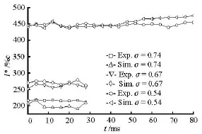
Fig.7 Relative cavity length at different cavitation numbers

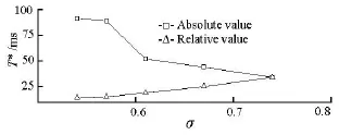
Fig.8 Reverse movement cycle of the two-phase interface at different cavitation numbers

Moreover， a reverse motion of the water-vapor mixture phase occurs within the cavity in all stages. The results show that the frequent exchange between the water phase and the vapor phase still exists inside the cavity， despite the fact that the cavity is already enclosed and that the cavitation contour line is relatively stable. The motion of the interface between the vapor phase and the water-vapor mixture is seen as the variation of the two-phase volume fraction inside the cavity. The cavity length is smaller with σ=0.74and σ=0.67. The water-vapor two-phase interface reverses to the hydrofoil end from the back of the cavity with a relatively short period， whereas the process lasts up to 92 ms until σ=0.54. For convenience of comparison， one reverse motion period is defined as the period when the two-phase interface starts to move from the cavity back to the hydrofoil leading point. Figure 8 shows thereverse movement cycle of the two-phaseinterfacefordifferentcavitationnumbers.The reverse movement period obviously increases with the decrease of the cavitation number （shown as absolute values）， and a sharp change occurs between the cavitation numbers 0.61 and 0.57. For various cavity lengths with different cavitation numbers， a relative backward motion cycle， T*， is defined as the original period multiplied by the cavity length at σ=0.74，and then divided by the cavity length at the current cavitation number， which is also given in Fig.8 （shown as the relative value）. It can be shown that the relative adverse motion period sees a linear decrease with the decreasing cavitation number. This trend shows that when the cavitation number continuously drops， the volume exchange and the mass transfer between the water and the vapor phases inside the cavity become increasingly frequent， resulting in more even supercavitating flows.

Fig.9 Transient pressure distributions

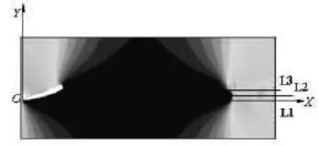
Fig.10 Schematic diagram of the special section location

2.2Pressure distribution

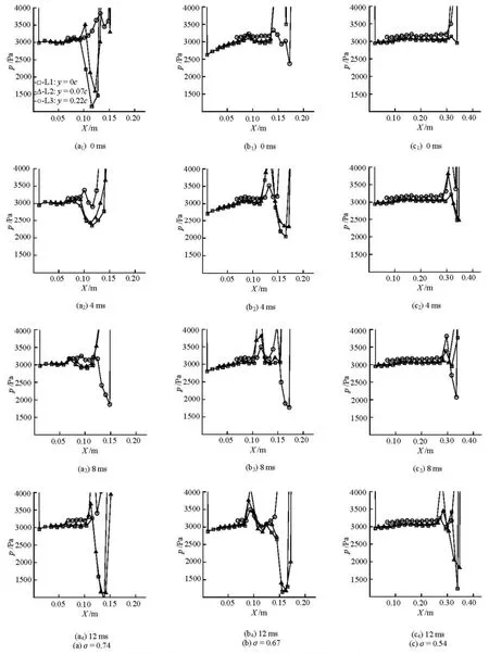
Fig.11 Instantaneous pressure distributions at the level sections

The dynamic pressure is obtained to understand the reverse motion mechanism of the two-phase interface in the cavity. Figure 9 shows the transient pressure distributions. A low pressure area appears behind the hydrofoil suction surface in all stages （shown in black color）， and extends downstream with the reduction of the cavitation number. Unlike the mainstream area with high pressure （shown in gay color）， thepressure fluctuation near the wake of the low pressure region and the vortex entrainment make the local vortex to have an instantaneous variation， which behaves as the periodic shedding of the upper and lower vortices （corresponding to the cavitation structures in Fig.6）. For example， as shown in Fig.9 with σ=0.74， at =0mst， the upper vortex near the cavity tail occupies a dominant position， which rotates in a clockwise direction （shown in red arrow）， at =4mst， the lower vortex is much stronger， which rotates in a counterclockwise direction （indicated with arrows）， then a periodic vortex shedding forms. The similar behavior can be seen in the case of σ=0.67and σ=0.54. As a result of adverse pressure gradient effects， some of the upper and lower vortices near the cavity enclosing point begin to shed downstream， whereas others move reversely toward the cavity front， resulting in a dynamic distribution of the water-vapor mixture phase in the cavity.

To further reveal the pressure distribution characteristics in the supercavitation region， Fig.10 gives the position of three relative level sections， wherein the hydrofoil leading vertex is chosen as the coordinate origin， and three ordinate points are fixed: the hydrofoil leading vertex with =0y， the middle point of the suction surface with y=0.069c， and the trailing edge vertex with y=0.222c. Figure 11 gives the transient pressure variation in the corresponding positions，where the reference vaporization pressure is 3 168 Pa. Apparently， in all cases: （1） Corresponding to the cavity tail， one position exists at which the pressure dramatically decreases to a level below the vaporization pressure and reaches a minimum value， then back around the vaporization pressure. The same pressure variation trend occurs at the sections of L1 and L2，whereas the opposite occurs at the L3 section. Obviously， it corresponds to the alternate shedding of the upper and lower vortices formed at the cavity tail，where the change of the vortex-core position results in the variation of the lowest pressure location. （2） Violent pressure fluctuation occurs at some place inside the cavity， the local pressure can be seen to suddenly increase and exceeds the vaporization pressure， then rapidly decreases to a certain level near the latter. The fluctuation surface moves reversely along with time. A comparison with the above vapor volume fraction distribution demonstrates that the pressure fluctuation position corresponds exactly the water-vapor twophase interface location， and the reverse movement of the pressure fluctuation position results in the adverse motion of the two-phase interface. The pressure suddenly increases because a pure vapor region is formed in front of the two-phase interface， where the liquid is completely vaporized. （3） Compared with the watervapor mixture area at the back of the cavity， the pressure in the vapor area is inversely and slowly reduced，having a minimum value near the suction side. Moreover， the pressure distribution is more uniform in the vapor area because the frequent volume and mass transfers in the water-vapor mixture area results in a continuous pressure fluctuation. （4） At the vertical direction in the cavity， the pressure gradually increases from the L1 section to the L3 section， i.e.， the upper pressure is always greater than the lower pressure in the cavity.

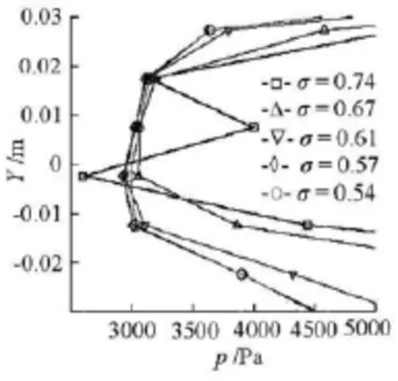
Fig.12 Pressure distributions on the vertical sections

To better display the pressure variation perpendicular to the flow direction， the relative instantaneous pressure distribution at the vertical section of =1.4xc is obtained based on the coordinates mentioned above， as shown in Fig.12. Except at σ=0.74 （in the wake region）， the pressure in the mainstream area gradually decreases with the decreasing cavitation number， while behaving relatively stable in the cavitation region. Moreover， a great pressure gradient exists in the cavity boundary. Figure 13 shows the transient pressure distributions on several vertical sections for various cavitation numbers. The cavity length is shorter at =σ 0.74， hence the latter two sections （=1.5xc and =x 2.0c） are located in the wake region， where the local pressure dramatically decreases. However， the same characteristics can be found in all stages: （1） the minimum pressure position is obtained within the shear layer， beginning from the foil leading point （=0）x. A strong shear layer forms from the hydrofoil leading vertex because of its special structure. The continuous vortex motion in the shear layer leads to a local pressure reduction. （2） At every vertical section， the pressure monotonously increases from the shear layer to the upper part of the cavity. （3） A large pressure gradient exists near the upper and lower boundaries of the cavity， which indicates that the cavitation boundary is located at the position where the pressure sharply increases. The cavitation region expands with the decreasing cavitation number， whereas the pressure gradient at the boundary is gradually reduced.

Fig.13 Instantaneous pressure distributions on the vertical sections

3. Conclusions

The flow characteristics in different supercavitating regimes around a hydrofoil are simulated through a related numerical model. The reverse motion mecha-nism of the interface between the water and vapor phases is analyzed based on the cavitation structure and the pressure distribution. The following is a summary of the main findings:

（1） A reverse motion of the water-vapor mixture phase occurs within the cavity in all supercavitating stages. The relative adverse motion period sees a linear decrease with the reduction of the cavitation number. This result shows that when the cavitation number drops continuously， the volume exchange and the mass transfer between the water and vapor phases inside the cavity become more frequent， resulting in a more even supercavitating flow.

（2） The effect of the adverse pressure gradient induces the adverse pressure fluctuation inside the cavity. Corresponding to the two-phase interface position inside the cavity， a violent pressure fluctuation occurs. This fluctuation can be observed from the local pressure that suddenly increases and exceeds the vaporization pressure， then rapidly decreases to a level near the latter， the fluctuation surface moves reversely along with time. In short， the variation in the pressure fluctuation position results in a reverse motion of the two-phase interface in the cavity.

（3） Compared with the water-vapor mixture area at the back of the cavity， the pressure in the vapor area becomes inversely and slowly reduced， with a minimum value near the suction side. Unlike the mainstream area， a higher pressure gradient occurs near the cavity boundary， and the minimum pressure position is related to the shear layer beginning from the foil leading point.

In this paper， we mainly focus on the qualitative analyses of the flow structure and the pressure distribution in the cavity. The adopted parameters including the inlet velocity， the chord length and the lift angle of the foil are all constants. In a future research， the systematic simulation will be carried out under different conditions， and some experimental means will be considered to directly obtain the pressure distribution， the quantitative variation will further reveal the mechanism of the reverse flow in the supercavitation region.

Acknowledgements

The sponsoring of the China scholarship fund，the Beijing Key Laboratory of Passive Safety Technology for Nuclear Energy is gratefully appreciated.

References

［1］WANG G.， CAO S. and IKOHAGI T. Study on behaviors of cavitating vortices in flows around a hollow-jet valve［C］. Third International Conference on Fluid Machinery and Fluid Engineering. Beijing， China， 2000， 451-455.

［2］WANG G.， SENOCAK I. and SHYY W. et al. Dynamics of attached turbulent cavitating flows［J］. Progress in Aerospace Sciences， 2010， 37（6）: 551-581.

［3］WEILAND C.， VLACHOS P. P. Time-scale for critical growth of partial and supercavitation development over impulsively translating projectile［J］. International Journal of Multiphase Flow， 2012， 38（1）: 73-86.

［4］KIM Seon-Hong， KIM Nakwan. Hydrodynamics and modeling of a ventilated supercavitating body in transition phase［J］. Journal of Hydrodynamics， 2015， 27（5）: 763-772.

［5］PAN Zhan-cheng， LU Chuan-jing and CHEN Ying. Study on the characteristic of a forced pitching supercavitating vehicle［J］. Journal of Shanghai Jiaotong University（Science）， 2015， 20（6）: 713-720.

［6］LIU Tao-tao， WANG Guo-yu and DUAN Lei. Assessment of a modified turbulence model based experiment results for ventilated supercavity［J］. Transactions of Beijing Institute of Technology， 2016， 36（3）: 247-251（in Chinese）.

［7］KARIM M. M.， AHMMED M. S. Numerical study of periodic cavitating flow around NACA0012 hydrofoil［J］. Ocean Engineering， 2012， 55（15）: 81-87.

［8］ZHI S. Numerical investigations of supercavitation around blunt bodies of submarine shape［J］. Applied Mathematical Modelling， 2013， 37（20-21）: 8836-8845.

［9］WOSNIK M.， ARNDT R. E. A. Measurements in high void-fraction bubbly wakes created by ventilated supercavitation［J］. Journal of Fluids Engineering， 2013，135（1）: 011304.

［10］ SHAFAGHAT R.， HOSSEINALIPOUR S. M. and NOURI N. M. et al. Shape optimization of two-dimensional cavitators in supercavitating flows， using NSGA II algorithm［J］. Applied Ocean Research， 2008， 30（4）: 305-310.

［11］ RASHIDIAI.，PASANDIDEH-FARDA M. and PASSANDIDEH-FARD M. et al. Numerical and experimental study of a ventilated supercavitating vehicle［J］. Journal of Fluids Engineering， 2014， 136（10）: 101301.

［12］ LI X.， WANG G. and ZHANG M. et al. Structures of supercavitating multiphase flows［J］. International Journal of Thermal Sciences， 2008， 47（10）: 1263-1275.

［13］ TULIN M. P. Supercavitating propellers［C］. Proceedings of Fourth ONR Symposium on Naval Hydrodynamics. Rhode-Saint-Genese， Belgium， 2001， 239-286.

［14］ LI Xiang-bin， WANG Guo-yu and YU Zhi-yi et al. Multiphase fluid dynamics and transport processes of low capillary number cavitating flows［J］. Acta Mechanica Sinica， 2009， 25（2）: 161-172.

［15］ OLIVER C. D.， FORTES P. R. and REBOUD J. L. Evaluation of the turbulence model influence on the numerical simulations of unsteady cavitation［J］. Journal of Fluids Engineering， 2003， 125（1）: 38-45.

［16］ SCHNERR G. H.， SAUE J. Physical and numerical modelling of unsteady cavitation dynamics［C］. The 4th International Cconference on Mmultiphase Flow. New Orleans， USA， 2001.

［17］ SINGHAL A. K.， ATHAVALE M. M. and LI H. Y. et al. Mathematical basis and validation of the full cavitation model［J］. Journal of Fluids Engineering， 2002， 124（3）: 617-624.

［18］ LI Xiang-bin， WANG Guo-yu and ZHANG Bo et al. Evaluation of the RNG -kε model on the numerical simulations of supercavitating flows around a hydrofoil［J］. Chinese Journal of Hydrodynamics， 2008， 23（2）: 181-188（in Chinese）.

（May 21， 2014， Revised August 18， 2014）

* Project supported by the National Natural Science Foundation of China （Grant No. 50679001）.

Biography： Xiang-bin LI （1975-）， Male， Ph. D.， Lecturer