Jianming YANG

Fidesi Solutions LLC， PO Box 734， Iowa City， IA 52244， USA， E-mail: jmyang@fidesisolutions.com

Sharp interface direct forcing immersed boundary methods：A summary of some algorithms and applications*

Jianming YANG

Fidesi Solutions LLC， PO Box 734， Iowa City， IA 52244， USA， E-mail: jmyang@fidesisolutions.com

Body-fitted mesh generation has long been the bottleneck of simulating fluid flows involving complex geometries. Immersed boundary methods are non-boundary-conforming methods that have gained great popularity in the last two decades for their simplicity and flexibility， as well as their non-compromised accuracy. This paper presents a summary of some numerical algori- thms along the line of sharp interface direct forcing approaches and their applications in some practical problems. The algorithms include basic Navier-Stokes solvers， immersed boundary setup procedures， treatments of stationary and moving immersed bounda- ries， and fluid-structure coupling schemes. Applications of these algorithms in particulate flows， flow-induced vibrations， biofluid dynamics，and free-surface hydrodynamics are demonstrated. Some concluding remarks are made， including several future research directions that can further expand the application regime of immersed boundary methods.

immersed boundary methods， direct forcing sharp interface method， strong coupling schemes， fluid-structure interactions， Cartesian grid methods

Introduction

Body-fitted mesh generation has long been the bottleneck of simulating fluid flows involving complex geometries. Generating a body-fitted structured grid usually requires a great amount of user inputs. It is very time-consuming and the grid quality heavily depends on the user's gridding expertise and understanding of the flow physics to be studied. Automated body-fitted mesh generation algorithms can greatly reduce human work， but the algorithm robustness and mesh quality for real world complex geometries are still of major concern to users. Many meshless methods， such as vortex methods［1］， smoothed particle hydrodynamics （SPH）［2］， etc.， aiming at eliminating the meshing needs were developed in the literature. Unfortunately， in a meshless method a “point generation” strategy similar to an unstructured mesh generation process is still required and point clouds have to be defined，which essentially establish connections locally among the seemingly globally unconnected points. Defining a point cloud and operating upon it for solving the governing equation are highly complicated processes，which make it very hard to develop efficient solution algorithms. Moreover， it is very difficult to achieve good conservative properties with meshless methods. On the other hand， non-boundary-conforming methods rely on mostly simple Cartesian grids that can be generated trivially for covering the whole computatio- nal domain including embedded geometries. Immersed boundary methods （IBM） are non-boundary-conforming methods that have gained great popularity in the last two decades for their simplicity and flexibility， as well as their non-compromised accuracy. It is worth noting that sometimes cut cell methods［3，4］were categorized as IBM in the literature. However， the grids in cut cell methods are unstructured meshes in the sense that the solid boundaries are retained to form bodyfitted irregular cells together with the regular grid lines/faces. Different irregular cells need different treatments or， a generic treatment similar to what in an unstructured mesh solver has to be followed， which makes the cut cell methods very complicated and prone to robustness issues， especially for 3-D problems. These difficulties are also evidenced by the merely sporadic studies of 3-D cut cell methods in the literature.

Here we are concerned with the IBM originated by Peskin in the last seventies［5，6］for the computational studies of fluid-structure interaction （FSI） problems in a human heart. In Peskin's method［7］， the effect of flexible structures on the fluid flow was represented by an external， singular force field in the Navier-Stokes equations to be solved in a regular domain including both the flow field and the structures. The structural deformation that is described in a Lagrangian framework was modeled by a constitutive relation for the material elasticity. Due to the mismatched spatial discretizations， usually a discrete delta function was used as the kernel for connecting the fluid flow and the immersed flexible structures， that is， to interpolate the fluid velocity from the Eulerian grid points to the Lagrangian elements and to spread out the boundary forces from the latter to the former. Structures with no/prescribed deformations can be modeled as elastic materials of very large stiffness. However， the material stiffness has to be determined ad hoc or adjusted during a computation. For example， in Ref.［8］ the local forcing function modeling the structural effect on the fluid flow would adapt itself through a feedback controller to satisfy the desired velocity boundary conditions. Also， this feedback forcing strategy was implemented in a finite difference method［9］， instead of the pseudo-spectral method in Ref.［8］， for simulating low Reynolds number flows past stationary and moving circular cylinders. A major problem with the feedback forcing method is that the feedback mechanism contains two large-magnitude adjustable constants， which make the whole system very stiff and time step has to be greatly reduced.

Without relying on a constitutive relation for linking the material elasticity （thus structural deformation）and the singular force density， Mohd-Yusof［10］derived the momentum forcing function directly by imposing the velocity boundary condition at the immersed boundary in the discrete-time equations without any feedback adjustment， thus comes the name “direct forcing”approach. It was implemented in a pseudo-spectral method in Ref.［10］ and then applied in a finite difference method by Fadlun et al.［11］. With Mohd-Yusof's derivation， the direct forcing approach can be viewed as a local solution reconstruction procedure to satisfy the desired boundary conditions at the immersed boundary and an explicit forcing term was not even required in the momentum equations at all［11］. Because the velocity boundary conditions are ubiquitous in numerical simulations of fluid flows regardless of the boundary properties （rigid， deforming， or elastic） and the motion characteristics （stationary， prescribed， or predicted）， the direct forcing formulation opened up great opportunities for developing algorithms of various features targeted for specific improvements as well as diversified applications.

Initially the development and applications of the direct forcing approach were focused on stationary immersed boundaries （see， for example， Refs.［11-14］among others）. In these studies， the momentum forcing functions were determined discretely and applied to grid points （either in the fluid or the solid phase） immediately next to the immersed boundary， without drawing support from a smoothed delta function to spread out the forcing to more neighboring points as in Peskin's formulations. For moving boundary problems， the material property of a grid point near the immersed boundary may change from fluid to solid in one time step， and vice versa. The role switches of grid points due to a moving boundary on a fixed grid have some implications in a time-splitting scheme， such as the fractional-step method， and may result in large spurious oscillations in the time histories of hydrodynamic forces. Uhlmann［15］mitigated the spurious force oscillation problems by combining the discrete delta function kernels with the direct forcing formulation， such that the momentum forcing can be spread out over a few grid points across the immersed boundary. In Uhlmann's approach， the Eulerian velocities at grid points surrounding the immersed boundary were first interpolated to a Lagrangian node on the immersed boundary using the discrete delta function. Then， instead of using a constitutive law or feedback adjustment， the local forcing is determined by directly requiring the velocity boundary condition at the boundary node to be satisfied after the forcing is applied. Finally the local forcing at each boundary node is distributed using the discrete delta function to surrounding grid points. Similar Eulerian-Lagrangian coupling ideas in the direct forcing framework were also presented in Ref.［16］ with a Lattice Boltzmann method and Ref.［17］with a bilinear interpolation/extrapolation scheme. Uhlmann's method has been widely used in particulate flow simulations and inspired quite some follow-up work for further improvements or extensions to general FSI problems， such as Refs.［18-21］ among others. However， there are several inherent drawbacks of using discrete delta function kernels in IBM. For instance， the smoothing process results in a blurring fluid-solid interface as well as an increased computational cost， depending on the width of the support of the delta function on the Eulerian grid. Also， the Lagrangian markers on the immersed boundary are usually required to be distributed evenly with a resolution close to that of the local Eulerian grid （a finer surface mesh will increase the cost， instead of the accuracy）［15］， even for stationary geometries or structures with prescribed motions. This could be very difficult，if not impossible， for cases with complex geometries or thousands/millions of particles of arbitrary shapes. In addition， some ad hoc treatments［21］may be necessary if the Eulerian stencils from two different structures overlap.

Due to the abovementioned drawbacks， it is stillpreferred to avoid the dependence on a discrete delta function as the kernel of fluid-structure （i.e.， Eulerian-Lagrangian） coupling in many applications by retaining the sharp interface property of the original direct forcing approach［11］. But as discussed earlier， the sharp interface treatment may produce temporal and spatial jumps in the momentum forcing when the immersed boundary moves across the fixed grid points. Without an appropriate handling， these jumps can result in spurious oscillations of hydrodynamic forces on the immersed boundary， which could be disastrous for FSI problems sensitive to the variations in the hydrodynamic forces. As demonstrated in Ref.［22］， non-physical historical information may enter the flow field in a time step， when some grid points with reconstructed solutions at the previous time step become normal fluid points， if no treatment is applied to recover the correct historical information at these points. Ref.［22］proposed a field extension strategy that， at the end of each time step， the flow field is extended into the grid points with non-physical values near the immersed boundary through extrapolations.

In this work， some numerical algorithms developed along the line of the approach in Ref.［22］ will be summarized and their applications in some practical problems will be demonstrated. In particular， the Cartesian grid approach was extended to cylindrical coordinates in Ref.［23］， which can be very efficient for flows past axisymmetric bodies and/or （quasi-） solids of revolution. In Ref.［24］， an iterative strong coupling scheme was developed for simulating fluid- structure interaction problems within a sharp interface direct forcing （SIDF） approach. A comparison with a weak coupling scheme was shown to illustrate the necessity of using strong coupling schemes for their desirable robustness and applicability. In Ref.［25］ this strong coupling scheme was much improved in effi- ciency as the fluid flow was solved only once in each time step， although the structural displacements and velocities were still iteratively solved. Then in Ref.［26］ it was shown that such a sharp interface approach could be applied to particulate flow simulations with similar coarse grids as those in continuous forcing me- thods. Recently， in Ref.［27］ a non-iterative strong cou- pling scheme was proposed to further improve the computational efficiency. On the other hand， the IBM from Ref.［22］ was extended to deal with gas-liquid- solid systems including free-surface hydrodynamics in Ref.［28］. Fully coupled simulations of wave-body interaction problems were also demonstrated in Ref.［29］using a non-inertial reference frame. In addition， a triangulation setup procedure for immersed boundary simulations was reported in Ref.［30］. This topic was usually overlooked in the IBM literature， but a robust and efficient procedure is very important for the applicability of IBM in practical problems， especially when FSIs are involved.

1. Numerical algorithms

1.1Fluid flow solvers

It is necessary to decide the frame of reference before introducing the governing equations. Both inertial and non-inertial reference frames can be used in immersed boundary simulations. The simplest choice is an inertial reference frame fixed to or moving at a constant velocity with respect to the earth. With such an inertial reference frame， the incompressible viscous flows are governed by the Navier-Stokes equations:

where u is the velocity vector， p is the pressure， g represents the gravitational acceleration， ρ is the density， t is the time， I is the unit tensor， and T is the viscous stress tensor defined as

with μ the dynamic viscosity， S the strain rate tensor given by

where the superscript T represents transpose operation. Spatial filtering can be applied for large-eddy simulation （LES） of turbulence， then in the equations above the velocity vector and pressure become the corresponding spatial filtered variables and μ represents the total effective viscosity， i.e.， the sum of the molecular and eddy viscosity. These equations can be applied to multi-phase flows， but for direct numerical simulation （DNS） of single-phase flow with constant density and viscosity， the momentum equation can be much simplified as

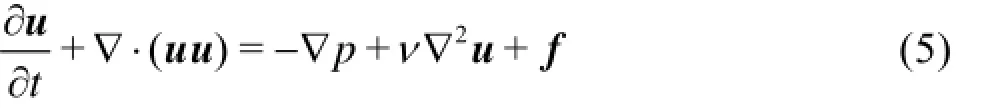
with ν the kinematic viscosity of the fluid， the density ρ as a constant absorbed into the pressure p，and f the body force including the momentum forcing term from the immersed boundary treatment. For simplicity， Eq.（5） will be used for the momentum equation hereafter unless declared explicitly. On the other hand， it may result in more efficient algorithm and/or can be more convenient to adopt a non-inertial reference frame fixed to an immersed body that under-goes an unsteady large-amplitude motion including rotation. The conservative form of the governing equations in a non-inertial reference frame can be found in Refs.［31，32，27］.

A simple finite difference method can be used to discretize the Navier-Stokes equations on a non-uniform staggered Cartesian grid. For incompressible flows considered here， second-order central difference scheme （CDS） can be applied if the grid resolution is fine enough. Otherwise， upwind schemes need to be applied to enhance the numerical stability of the solver. A frequently used one is the third-order quadratic upwind interpolation for convective kinematics （QUICK）scheme［33］. The numerical stability and also accuracy can be further enhanced by using the fifth-order weighted essentially non-oscillatory （WENO） scheme［34］. For discretization of the viscous terms and the pressure gradient， standard second-order central difference schemes can be used. Second-order semi-implicit or fully explicit schemes can be used in time advancement of the momentum equation. The semi-implicit scheme gives the second-order Crank-Nicolson scheme for the diagonal viscous terms and the second-order Adams-Bashforth scheme for the convective terms and other viscous terms； whereas the latter will be applied to both convective and viscous terms in the fully explicit time advancement. For low Reynolds number flows， the viscous terms may give a more restrictive constraint on the time step than that from the convective terms， and a semi-implicit scheme can greatly relieve this constraint. Then the approximate factorization method［35］can be used to invert the momentum equations by solving three tridiagonal linear equations. With domain decomposition for parallelization， the matrix of each tridiagonal system will be distributed over a number of processors. Iterative solvers can be used by solving the sub-system in each block and then updating the ghost cells. However， the performance is not optimal and an extra convergence error will be introduced. Some parallel tridiagonal system solvers have been developed， the one given in Ref.［36］ has been proved to be efficient and robust. A fractionalstep method［37］can be employed for the velocity-pressure coupling， in which a pressure Poisson equation has to be solved to enforce the continuity equation. The pressure Poisson equation can be solved with the semicoarsening multigrid solver SMG in the Hypre library developed at Lawrence Livermore National Laboratory［38］. This multigrid solver is very efficient and highly scalable on massively parallel machines， which is essential for large-scale simulations. It is also possible to solve the pressure Poisson equation with direct methods［39］. The direct solver is very efficient， but requires the fluid density to be a constant and the use of a uniform grid in one coordinate direction for 3-D problems.

1.2Immersed boundary setup procedures

In general， an immersed boundary doesn't coincide with the grid points on the underlying grid. Its geometric information， together with the boundary conditions， has to be reflected on the Eulerian grid through some immersed boundary setup procedures. Both Eulerian and Lagrangian representations can be used for the description of the immersed boundaries. But a Lagrangian representation is more memory efficient and the motion of the solid object will not introduce any distortion or volume loss. Usually the triangulated surface is specified in the body-fixed noninertial frame. For moving boundary problems， a transformation involving a linear and angular displacement is applied at each time step to obtain the current immersed boundary in the inertial frame.

1.2.1Immersed boundary description

For simple geometries such as cylinder， sphere，and other frequently used primitives in computer aided design （CAD）， implicit surfaces by analytical functions can be used. For a circular cylinder or a sphere，which is frequently used in immersed boundary simulations， the only information needed is the center and radius of the geometry. Sometimes parameterized curves/surfaces can be simple and efficient choices. For general complex geometries， however， surface meshes（usually with triangular elements） are the most popular choice due to the well-balanced simplicity and efficiency. Surface triangulations can be used to represent arbitrary geometries， either open or closed， solid or deformable， separated or interconnected.

Many different file formats （or data structures）exist for representing surface triangulations. The stereolithography （STL） format is a very simple format and available from major CAD software packages. It stores a triangulated surface using the unit normal and three vertices of each triangle in Cartesian coordinates. For a valid solid that is watertight， the normal vectors can be used to define the inside/outside of solid. One major issue of STL format for IBM applications is that the STL files from various sources may contain errors such as holes， cracks， and triangles with wrong normal vectors. In addition， a STL file stores many redundant vertices， as each element is stored as three independent vertices without any connectivity or topology information.

A finite element surface triangulation gives the numbers of unique vertices and triangles， together with a list of vertex coordinates and a list of triangles （indices of the three vertices）. Basically， the format is the most memory-effective one. But same as the STL format， it does not give topology information. Due to the lack of adjacency table， consistent treatment of neighboring triangles during the geometric operations is difficult to achieve.

The GTS format as defined in the GNU triangulated surface （GTS） Library［40］seems to be a good choice for the setup procedure. A GTS file consists of the numbers of vertices， edges， and faces （triangles）followed by the lists of vertices， edges （vertex indices），and faces （edge indices）. The edge connectivity information extra to the two formats discussed above can be very useful for robust geometric operations. The GTS Library is an Open Source Free Software library，which provides a set of useful functions to deal with 3-D surfaces meshed with interconnected triangles. The package also provides useful conversion utilities between GTS format and other widely used CAD formats including STL.

There are other file formats for surface triangulations with complete vertex， edge， and face adjacency information. However， additional information is usually not required for the basic geometrical operations involved in IBM applications.

A salient feature of the SIDF-IBM presented here is that the resolution of a triangulation can be solely determined according to the desired level of surface feature preservation， regardless of the resolution of the Eulerian grid to be used for the simulation. For example， a cube can be perfectly described by 12 triangles as shown in Ref.［26］， and more surface triangles only increase the required memory and CPU time for processing without any benefits. This is quite different from those approaches that utilize a discrete delta function as the kernel for the Lagrangian-Eulerian coupling or calculate the fluid force by integrating the surface pressure and shear stress， and the present one is generally much simpler and more efficient.

1.2.2Inside/outside status determination

After the Lagrangian description of the immersed boundary is given， the relation between the immersed boundary and the underlying Eulerian grid can be determined. For a solid object that can be described analytically， usually the relative position of a point with regard to the solid can be determined analytically. For example， the status of a point can be easily given as inside or outside of a sphere， if the distance from this point to the center of the sphere is smaller or larger than the radius of the sphere， respectively. For a thin object such as a 2-D filament or a 3-D membrane， it only needs to locate the intersections of the grid lines with the thin object. But for a solid object with an internal space， usually the grid points inside the solid have to be identified for various purposes. Because the“line-segment intersection” （2-D） and the “line-surface intersection” （3-D） are relatively straightforward geometrical operations， here we only consider an immersed object that is a closed， watertight manifold and well resolved by the underlying grid.

The inside/outside status of a grid point with regard to a watertight triangulation can be determined through the so-called “point in polyhedron” algorithm. That is， to cast a ray from a point and count the number of intersections of this ray with the triangulation. The core geometric operation will be the “segmenttriangle intersection” test in 3-D as discussed in Ref.［41］. For Cartesian grids， all grid lines align with the coordinate directions， thus grid points along a grid line can share the same ray for this purpose［42］. It is also evident here that these algorithms can be used for thin membranes as mentioned above. The “segmenttriangle intersection” test for the inside/outside status determination of all grid points can be implemented in a straightforward manner.

By taking advantage of the fact that all grid lines in a Cartesian grid are parallel to one of the three axes，a simple and efficient 2-D “point-in-triangle” test is used to replace the 3-D “line-triangle intersection” test for calculating the intersections of a grid line with the triangulation. Hence， the inside/outside status of all points on this grid line can be easily determined. Since a coordinate-aligned line is to be used as a ray， for the intersection of the line with the plane that the triangle lies within， two of three coordinates are already specified. By utilizing the linear property of a triangle， the third coordinate can be evaluated using the barycentric coordinates of the point （line/ray in 3-D） with regard to the 2-D projection of the 3-D triangle. Compared with the 3-D “line-triangle intersection” test， the 2-D“point-in-triangle” test only uses one third floating operations， which represents a substantial savings in computational cost for cases with high resolution Cartesian grids and fine surface triangulations.

One major issue that affects the robustness of geometric algorithms is the inaccuracies in floating point arithmetic. For instance， a point very close to an edge of a triangle may be determined as outside， but it could be calculated as outside for the neighboring triangle that shares the same edge with the former triangle due to the floating point error. In addition， for cases with an intersection coinciding with a vertex or on one of the edges， this intersection may be countered multiple times for all triangles sharing the same vertex and twice for two triangles sharing the same edge. These issues have to be considered adequately in the solver.

1.2.3Grid point classification

Grid point classification for the immersed boundary treatment is performed after the inside /outside status of all grid points is determined. Here， as shown in Fig.1， a grid point inside the solid body is tagged as a solid point； a grid point is tagged as an interface point if it is in the fluid phase （outside the solid bodies）and one or more grid line segments linking it to its immediate neighbors are intersected by the immersed interface， all the other grid points are tagged as fluid points. Both the solid points and interface points are also collectively defined as forcing points for conve-nience， since the forcing term is imposed on all forcing points to represent the effect of an immersed rigid body on the fluid flow in our SIDF-IBM.

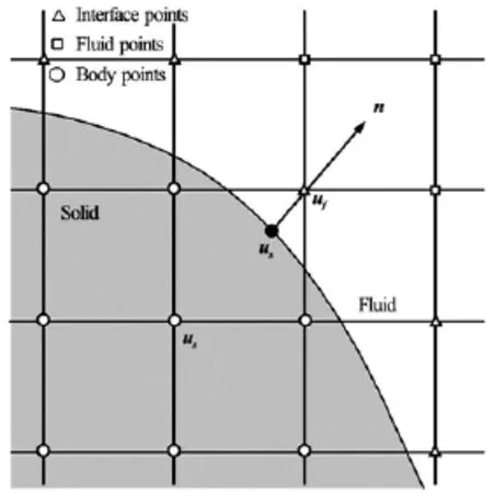
Fig.1 Grid point classification. Grey region is covered by the solid object

1.2.4Sub-cell position computation

To precisely apply the boundary conditions at the immersed boundary through the underlying grid， it is necessary to determine the relative position of the immersed boundary with respect to an interface point. There are two frequently used formulations: one is to obtain the sub-cell distances of an interface point to the immersed boundary along the grid lines， just like the 1-D approach adopted in Ref.［11］， the other is to obtain the closest point on the immersed boundary to the interface point， e.g.， the multiple dimensional scheme used in Ref.［14］ that has been widely accepted.

For a surface triangulation， the normal projection of an interface point is the closest point， which could be inside a triangle， on a triangle edge， or simply a triangle vertex. An intuitive implementation of this task is to loop over all triangles for each interface point and calculate the closest surface point on the triangle， if this interface point is within a slightly enlarged bounding box of the triangle under consideration. This grid-based closest surface point calculation approach is very simple and works fine for immersed objects with small number of triangles. However， for high-resolution simulations with complex geometries，triangulations with millions of faces could be encountered. This approach will be extremely expensive and the situation will be worse if FSIs with large-amplitude body motions are considered.

Actually， an efficient triangulation-based algorithm can be used for obtaining the closest surface point information for all interface points in one single loop of all triangles. For each triangle， a slightly enlarged bounding box is used similar to what given in the previous part. For all grid points within the bounding box， only those tagged as interface points will be fur- ther processed with closest surface point calculation. The local shortest distance to the triangle will be saved and the minimum value will be obtained after the loop over all triangles is completed. The global closest surface point on the triangulation corresponding to the global shortest distance will be stored for further usage. Again， like the ray-casting algorithm， some additional temporary storage is required for this triangulationbased closest surface point calculation algorithm. In the 3-D “closest point on triangle to point” algorithm from Ref.［43］， the Voronoi feature regions of a triangle is used to determine which feature the orthogonal projection of the interface point is in， then the closest point is only evaluated with the corresponding feature region. The information of the closest points can be converted to a signed distance field， i.e.， a level set function for the immersed boundary， which can be very useful in many applications.

1.3Immersed boundary treatments

1.3.1Momentum forcing term

In IBM， both the kinematic and dynamic boundary conditions have to be satisfied at the fluid-solid interface， Γ. Denote the position vector of the origin of the body-fixed frame in the inertial frame as d， the angular velocity vector of the moving body about the origin of the body-fixed frame as BΩ， or Ω for simplicity， and RIBthe rotation matrix for a rotation from the inertial frame to the body-fixed one， the kinematic condition can be expressed as follows for the non-slip velocity boundary condition，

for any pointΓx at the interface. Also， a rigid body motion is imposed on the fluid enclosed by the fluidsolid interface. Hence Eq.（6） is to be satisfied at every pointsx in the solid phase. The dynamic boundary condition is given as

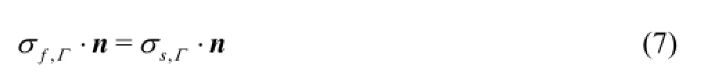
where σ is the stress tensor and n is the interface normal. This condition is automatically satisfied in the present method as the Navier-Stokes equations are discretized in the whole domain including the solid phase.

Let*u be the solution of the momentum equation. With the implicit Crank-Nicolson scheme for the viscous terms， the right-hand-side of the discretized momentum equation depends on u*and fn. Updating both u*and fniteratively is always possible，however， it is usually an inefficient choice. In Ref.［11］，a 1-D interpolation scheme was developed to directly incorporateinto the factorized linear system for u*， and fnwas not explicitly evaluated.

Here， the momentum forcing terms in different approaches are all obtained from the explicit solution of the momentum equation. With a fully explicit scheme the right-hand-side will be independent of * u， and fncan be calculated from Eq.（9） in a straightforward manner， as shown in Refs.［14，22，24］. The problem with a fully explicit scheme is that the time step could be very small due to the constraint from the viscous terms. In this work， similar to several previous studies［23，25，28］， a preliminary explicit step is carried out first［12］and Eq.（1） is discretized in time as follows:

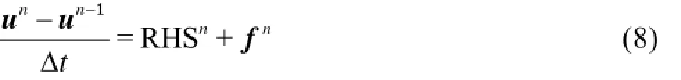
where RHS can be evaluated using the explicit firstorder Euler scheme or the second-order Adams-Bashforth scheme when possible. An explicit momentum forcing term can be derived from this formulation and it facilitates the selection of time steps based on the CFL condition alone， with a negligible viscous constraint in most cases. If the velocity boundary conditionis to be satisfied on the immersed boundary Γ， i.e. un=， the momentum forcing term fncan be determined as

For moving boundary problems， a rigid body motion is specified for the fluid enclosed in the immersed boundary. Therefore， Eq.（9） is also used to determine the momentum forcing term inside the immersed boundary， withreplaced by the solid velocityat the given location.

Apparently， for a grid point on the immersed boundary or inside the solid，nf can be evaluated directly without any problems. Unfortunately， it is not realistic to arrange grid points on a Cartesian grid to coincide with the immersed boundary for most， if not all， non-trivial applications. Therefore， the remaining question is how to impose the velocity boundary condition on an immersed boundary not aligning with the grid points. In Uhlmann's approach［15］， an interpolation using a discrete delta function was performed to obtain1n-u and RHS at a Lagrangian node on the immersed boundary， then the momentum forcing term could be evaluated there with Eq.（9）. On the other hand， as done in Ref.［11］， the velocity boundary condition can be satisfied through grid points close to the immersed boundary， provided that reasonable approximationsto the exact solutions unat these grid points can be obtained. Actually， an auxiliary velocity field can be derived from Eq.（8） with a zero momentum forcing term. It is evident that the momentum forcing term is zero for all fluid points in this approach. Therefore， the auxiliary velocity can be regarded as a good approximation to unon a fluid point. According to its definition， an interface point will be surrounded by fluid points and the immersed boundary. Therefore，a local reconstruction procedure is performed to getat an interface point utilizing the auxiliary velocity field at its neighboring fluid points and the immersed boundary velocityat the closest point of the interface point on the immersed boundary.

1.3.2Local reconstruction

The simplest approach is the 1-D linear interpolation as used in Ref.［11］. That is， for an interface point，there must be at least one grid line through it that intersects with the immersed boundary. The function value of this interface point will be the linear interpolation of the two function values at the intersection（i.e.， boundary condition） and the fluid point on the other side of the interface point. And if more than one grid lines go through the interface point， the interpolation can be performed along the one that gives the shortest distance between the intersection and the interface point. Of course， it is also possible to involve all grid lines that intersect the immersed boundary by using different weights along different grid lines， then the implicit treatment cannot be applied in a straightforward manner as in Ref.［11］.

In Ref.［14］ it was proposed to perform the interpolation along the normal direction of the immersed boundary. A probe point along the line normal to the boundary and through the interface point was identified first， and the local reconstruction was carried out between the boundary and the probe point along this line. For complex geometries with sharp corners， a well-defined normal direction may not be always available and the closest point to the interface point on the immersed boundary can be used as the normal projection of the interface point. One limitation of this approach is that the probe point is to be surrounded by fluid points， which may move the probe point away from the immersed boundary and result in a stencil of much wider support.

Actually， it is not necessary to require all grid points around the probe point to be fluid points as shown in Ref.［22］. This can easily achieved by placing the probe point within a grid cell， but on a specific plane passing through only fluid points. In a 2-D case，for example， two points on an x-grid line， y-grid line，or along the diagonal line will be checked to determi-ne that along which line both grid points are fluid points. Then the interpolation procedure is a singlestep process that involves two points from the fluid and one on the interface. The interpolation coefficients for the case of linear interpolation can be computed by solving 3×3 linear systems. For 3-D problems， 4×4 systems need to be inverted.

In Ref.［27］， the construction procedure of the interpolation stencils was reformulated to obtain a simple explicit expression and retain the desirable normal-oriented property and the grid point configuration as in Ref.［22］. These simple and compact formulations were easily derived referring to the straightforward geometric relationship. The degenerated 1-D and 2-D cases were also included. The explicit linear relationship between the immersed boundary velocity and the reconstructed flow velocity near the body can be used in fluid-structure coupling computations.

1.3.3Field extension

The field extension strategy was proposed by Yang and Balaras［22］for a sharp interface treatment in IBM for moving boundary problems. It was designed to fix the velocity and pressure derivatives at fluid points which were interface points at the previous time step， such that in the new time step all derivatives involved in the discretization at a fluid point contain physical values. This was implemented in Ref.［22］through an extrapolation procedure to directly modify the velocity and pressure solutions at some points that were determined based on their associations with interface/solid points. The field extension strategy is conceptually simple and practically effective as shown in Ref.［22，24］. However， the extrapolation procedure was not very convenient for complex geometries， also the modified solution fields made it difficult to express the momentum forcing term explicitly. Therefore， a simplified version was proposed in Ref.［25］ to avoid these drawbacks. The pressure derivatives， i.e.， the directional components of the pressure gradient， were directly used in the field extension operation， also， the velocity field extension was eliminated without impairing the overall accuracy.

1.3.4Force and moment evaluation

The total external force added to the flow field can be obtained from the integration of the momentum forcing term fn， i.e.，fndV . Consequently， the total external moment added to the flow field is simply（xn-dn）×fndV， with xnthe coordinates of a forcing point. Here both integrations are carried out over all forcing points （i.e.， interface and solid points）in a straightforward manner without involving any partial cell calculations. For example， the cell-wise force for a -ucomponent point （，，）ijk will be ρffx，ijkΔxiΔyjΔzkwith fx，ijkthe forcing term added to the u-momentum equation at this point.

The total external force and moment include what exerted on the fluid flow by the immersed body. In addition， the force and moment required for the portion of fluid occupied by the immersed body to do a rigid body motion arein the inertial frame andin the body-fixed non-inertial frame， respectively. Herefm is the mass andfI is the moment of inertia for the portion of fluid occupied by the immersed body. Therefore， the fluid force and moment exerted on a rigid body can be obtained by simply removing the rigid body motion portions， respectively.

1.4Fluid-structure coupling schemes

1.4.1Orientation representations

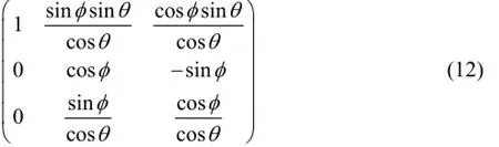
Two types of reference frames are usually used in FSI problems: an inertial reference frame fixed to or moving at a constant velocity with respect to the earth， and one or multiple non-inertial reference frames with each attached to one moving body under consideration. All fluid variables are conveniently defined in the inertial reference frame， whereas for a moving body， the motion can be described by the linear and angular displacements with respect to the inertial reference frame， and the linear and angular velocity with respect to the its own body-fixed non-inertial reference frame. The orientation of a solid body can be defined using the Euler angleT（，，）φθψ. Therefore， according to the -xyzconvention in the rotation order， the rotation matrixBIR can be written as

where c and s represent cos and sin functions， respectively.

The angular velocity Ω in the non-inertial reference frame can be related to the time rate of change of the Euler angles as follows

where Q is the transformation matrix given by

It is evident this equation fails for θ=±90o. This usually is not an issue for systems that are not designed to have such operational conditions. Nonetheless， two different systems of Euler angles can be adopted to avoid this singularity.

With the unit quaternion representation， the orientation of the body-fixed frame can be obtained from a rotation of angle α by the right-hand rule about an axis represented by a unit vector n =（nx，ny，nz）in the inertial frame. Then the unit quaternion representation for this rotation will be

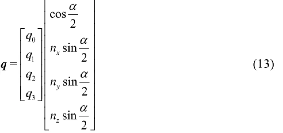
The time derivative of the quaternion is given by

The rotation matrixBIR for such a rotation from the inertial reference frame to the body-fixed one can be given as

The Euler angles can be obtained from the unit quaternion as follows:

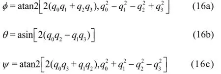
which can define the same rotation given by q according to the -xyzconvention in the rotation order， and the time rate of change of the Euler angles is related to the angular velocity Ω as given above.

1.4.2Rigid body dynamics

The dynamics of a rigid body in a fluid-structure coupled system is described by Newton's second law and Euler's equation， which are written in the inertial and the body-fixed non-inertial frames， respectively， as follows:

where sm is the mass of the solid body and sI is the moment of inertia of the body defined in the bodyfixed non-inertial frame.，（）rBrepresents the time derivative in the body-fixed non-inertial frame.IF and TBare the fluid force and moment in the inertial and the body-fixed non-inertial frames， respectively.，IeF represents all applicable external forces such as the gravitational force， spring and damper forces， and the collision force cF between solids. ，BeT represents all external moments from these external forces.

1.4.3ODE solvers

The dynamic equations for the rigid body motion，i.e.， Eqs.（17） and （18）， can be described as a set of standard first-order ordinary differential equations （ODEs）and solved using numerical integration schemes.

If fully explicit time advancement schemes are used， these ODEs can be integrated directly as demonstrated in Ref.［24］. Unfortunately， weak coupling schemes can be unstable for many problems， especially when the solid density is close to or smaller than the fluid density.

In Ref.［24］， Hamming's 4th-order predictor- corrector scheme is used to solve the governing equations for rigid body dynamics in a fully implicit manner. The equations for rigid body dynamics can be rewritten as a system of first-order ODEs. With Hamming's 4th-order predictor-corrector scheme， we have three steps: （1） predictor step， in which the solu- tion is explicitly predicted and then modified using the error estimated from the previous time step， （2） corrector step， in which the solution is corrected iteratively，and （3） finalizer step， in which the solution is updated using the estimated truncation error. This predictorcorrector scheme is very robust and efficient as shown in Ref.［24］.

In Ref.［27］， the trapezoidal rule was used for discretizing the force and moment in time， whereas allother terms were approximated using the second-order Adams-Bashforth scheme. The formulation for each solid body is quite similar to that in Ref.［32］ with the grid fixed to a single solid body. In Ref.［27］， however，a grid-parallel non-inertial frame attached to a solid body is only temporary and re-defined at each time step for each solid body in the domain， the actual solution of the rigid body dynamics equation is carried out in the permanent （i.e.， the global inertial and the bodyfixed non-inertial） frames for each solid body. With this strategy， the grid is decoupled from the motion of a single solid body， and arbitrary number of immersed bodies doing unlimited motions in the computational domain （i.e.， the grid） can be considered at the same time. For the quaternion evolution， usually higher order schemes are preferred for the accurate integration in a long run. The fourth-order Adams-Moulton scheme can be adopted， which is an implicit scheme capable of running at larger time steps and involves less work than the widely used explicit fourth-order Runge- Kutta scheme.

Fig.2 Three different strong coupling schemes

1.4.4Strong coupling schemes

The solution strategies for the coupled dynamics between fluid flow and structural response can be divided into two categories: monolithic and partitioned approaches. In the former， usually both sets of governing equations are solved with the same temporal and spatial discretization schemes and the fluid-structure coupling conditions are incorporated into the discretization and the resulting single linear system. Solution of this system gives both the flow field and the structural response. Whereas for the latter， there is no restriction with regard to the particular discretization schemes for either the fluid flow or the structural dynamics. However， compared with monolithic approaches， the numerical stability of partitioned approaches could be a more complicated issue.

Here we are only concerned with fluid-solid interactions and partitioned strong coupling approaches. Fig.2 shows the flow charts of three different strong coupling schemes to illustrate the similarities and distinctions among them. The first one is a global iterative scheme［24］. Except some explicit predictions only relying on information from previous time steps， all components are included in the iterative loop. At each time step， the iteration continues until the convergence criteria are met or the maximum number of iterations is reached. Such a global iterative strong coupling scheme is not particular to IBM， as which is also practiced in many boundary conforming approaches. Because the fluid flow solver is completely included in the loop， depending on the number of iterations， this strong coupling scheme can be much more expensive than a weak coupling scheme.

In Ref.［25］， a strong coupling scheme was developed with only a limited iterative loop that contains a few modules related to the immersed boundary setup procedure. Because the fluid solver is moved out ofthe loop， the strong coupling scheme in Ref.［24］ can be significantly expedited by several times or one order of magnitude. One main difference is that the fluid force and moment exerted on an immersed body can be evaluated by a simple pointwise integration of the momentum forcing term. Moreover， this step usually is applicable before solving the expensive pressure Poisson equation in a direct forcing framework. This step greatly simplifies the code structure and alleviates the memory requirement， but the strong coupling property of the FSI algorithm is not weakened at all.

Then in Ref.［27］， the iterative loop for fluid-structure coupling was completely removed. This was achieved with the help of temporary non-inertial frames. Each of them was designed to follow an individual immersed body， such that there is no relative motion between the grid and the solid body， and to be parallel to the inertial frame at the instant of previous time step， with a shift of the origin of the frame. Compared with the scenario in the inertial frame， it is evident that the position vector is not required in the present non-inertial frame. Kim and Choi［32］took advantage of this fact and the linear relationship in their IBM and developed a strong coupling algorithm for fluid-solid interaction problems with a single rigid body in a non-inertial frame. But with the scheme in Ref.［27］， many solid bodies can be packed together without interfering with the fluid-solid and solid-solid interactions. This procedure highly resembles a weak coupling scheme. The only difference is the introduction of a temporary grid-parallel non-inertial frame enabling an implicit direct solution of the rigid body dynamics instead of the fully explicit integration otherwise. The fluid flow and the motions of solid bodies are strongly coupled without involving any iteration between two systems of equations.

2. Applications

2.1Particulate flows

Fluid flows laden with solid particles are encountered in many engineering applications. The motion of a single particle in a fluid flow is often studied in order to understand the mechanism of the interactions between the solid particle and the fluid flow. Here a case studied in Ref.［44］， which was also used in Refs.［15］ and ［21］， is chosen for demonstration. The problem is configured as a spherical particle of diameter D settling to its terminal velocity V under gravity in an unbounded domain. In Ref.［21］ a series of simulations were conducted showing that their approach was stable down to a density ratio （ρs/ρf） around 0.3， which was a major improvement over the limitation of density ratio about 1.2 in the original approach［15］. With a discrete forcing function， the iterative predictor-corrector algorithm［25］was shown to be stable down to a density ratio of 0.29 in Ref.［30］. For the same test， the non-iterative strong-coupled scheme in Ref.［27］ can be stable with a minimum density ratio of 0.1 as shown in Fig.3. This case demonstrates the improved numerical stability as well as simplified code structure and increased computational efficiency with the non-iterative strong coupling scheme in Ref.［25］. Compared with the continuous forcing approaches in Refs.［15］ and ［21］ relying on complicated solid surface discretizations and expanded interpolation stencils， it can be very attractive even with the additional step of calculating the momentum forcing term in the noninertial frame.

Fig.3 Time histories of the settling/rising velocity of a spherical particle in a quiescent fluid with various low density ratios

The FSI problem of two drafting-kissing- tumbling particles is also frequently used in particulate flow simulations. As considered in Ref.［45］， two spherical particles of equal density and diameter descend under gravity， along with collision between particles， in a closed cuboid container filled with an incompressible viscous fluid. Here the computational setup was adopted from Ref.［45］ with some slight adjustments［30，25］. Figure 4 shows the instantaneous vortical structures around the particles in the course of settling as well as in sub-Figure （a） the centroid trajectories overlaid with particle instances corresponding to all other subfigures［25］. The particles are released at =0t in the still fluid. After they start to descend under gravity，the upper particle moves faster and is being “drafted”toward the lower one as the wake of the latter contains a downward velocity （Figs.4（b）-4（f））. The collision between the two particles happens near =0.33t. They keep a very small distance after collision for a while，which is called the “kissing” stage （Figs.4（g） and 4（h））. The upper particle descends to a similar height of the lower one in the “kissing” stage. Then individual wakes start to develop behind both particles along with increasing distance between them until they completely separate from each other， but still with interactingvortical wakes， near the end of this “tumbling” stage（Figs.4（i）-4（l））.

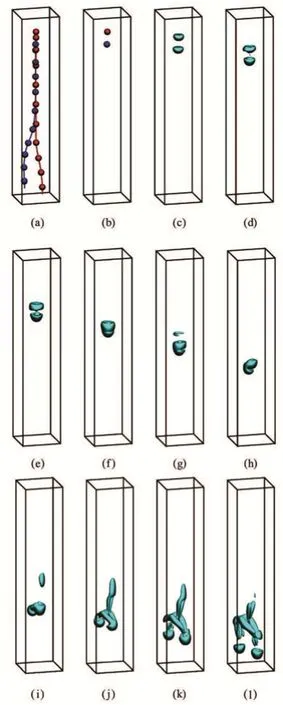
Fig.4 （Color online） Instantaneous vortical structures at several instants for two spherical particles settling in a quiescent fluid. （a） shows the trajectories

2.2Flow-induced vibrations

In Ref.［24］ the simulation of the vortex-induced vibrations of a periodic array of cylinders was demonstrated. This is a challenging problem for any type of boundary conforming formulation， since the presence of multiple bodies undergoing large displacements makes the preservation of the grid quality a very complex task. For IBM， grid generation is trivial since the boundary-conforming restriction is not there anymore. As a coupled problem， the motion of each body depends on the flow and indirectly on the motion of other bodies. It is a very stringent test for the robustness and efficiency of strongly coupled algorithms. Periodic boundary conditions were used in both coordinate dimensions and a constant flowrate was imposed. The resulting flow field is very complex compared to vortex-induced vibrations of a single cylinder. In Fig.5 vorticity contours for the 4×4 array are shown at one instant in time. Vortices originating from a cylinder upstream interact with the neighboring cylinders and other vortices generating a complex flow pattern.

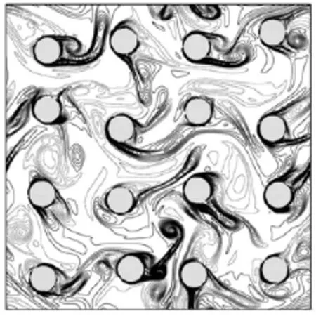
Fig.5 Vortex induced vibrations in a periodic 4×4 array of cylinders: Instantaneous vorticity contours

Galloping is a flow-induced structural motion characterized by low frequency， high amplitude oscillations. Here a case with two rectangular bodies undergoing galloping is demonstrated［25］: a transversely galloping body and a rotationally galloping body are placed in a free-stream in tandem arrangement. The Reynolds number is Re=UD/ν=250 with D the body thickness. The transversely galloping body has a square cross section （=1）Λ and the rotationally galloping body of a rectangular cross section gives =Λ 4 and is placed behind the square body with an initial distance 4.5D between the two centroids. Figure 6 shows several snapshots of the vorticity field around the bodies in the course of the upstream body heaving from the positive translational peak （a） to the negative peak position （e） and the downstream body pitching from the negative rotational peak （b） to the positive rotational peak position （f）. The deflection of the latter to the vortices shed from the former is evident. These deflected and elongated vortices interact with the vortices shed from the leading and trailing edges of the downstream body as they bypass it. In addition， their alternating circumvention above or below the downstream body restricts its galloping amplitude， and modulates its response frequency to be the same as that of the upstream body. These vortices then join those shed from the downstream body and are discharged in the combined wake.

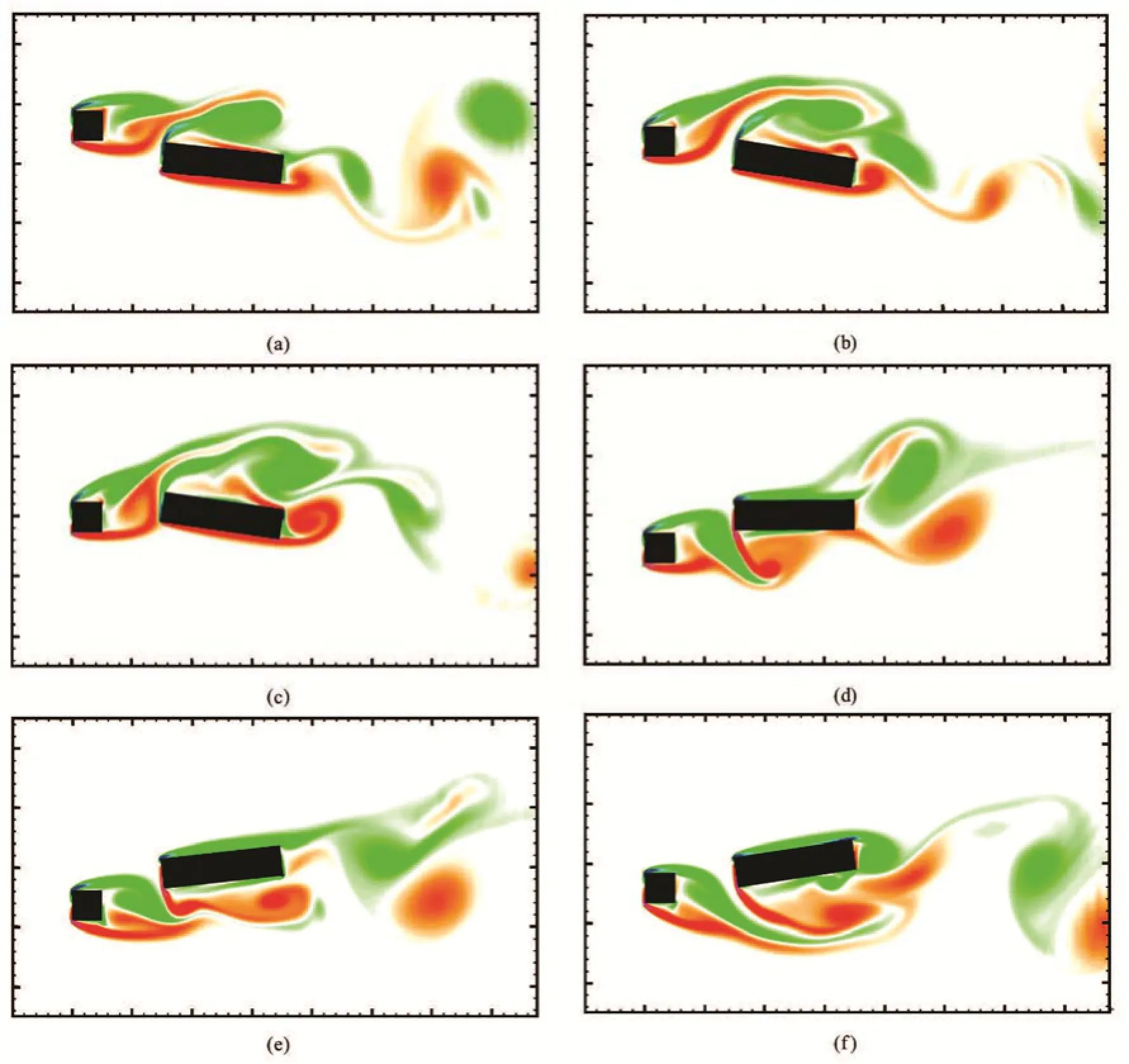
Fig.6 （Color online） Snapshots of the vorticity field around two rectangular bodies in tandem arrangement freely galloping in a freestream at Re=250

Flow-induced vibration problems exemplified above can be handled with body-fitted grids through grid deformation， regeneration， and/or overlapping， although substantially greater efforts are required in developing robust algorithms and maintaining the grid quality. As the complexity of the solid geometries， the number of structures involved， and/or the stiffness of the fluid-structure coupling increase， the difficulties in managing algorithm robustness and grid quality increase multifoldly. On the other hand， IBM can easily treat these increased complexities without posing any additional burden on the users for examining the grid correctness and quality.

2.3Biofluid dynamics

Andersen et al.［46］studied the quasi-2D aerodynamics of freely falling rectangular plates at intermediate Reynolds numbers in a water tank. Depending on the experimental parameters and initial conditions， a freely falling plate may experience fluttering （swinging from side to side）， tumbling （rotating and drifting obliquely）， or apparently chaotic motion with mixed fluttering and tumbling. For the case of a fluttering plate at Re=1147， a marginal grid resolution was used for resolving the thin plate with about 10 cells across the thickness direction. The plate develops a periodic fluttering motion very soon after it is released with the current initial angle. The plate swings from side to side during the free fall under gravity. It glides from a turning point on one side with low angle of attack （the angle between the direction along the plate width and its translational velocity vector at the center of mass）. Near the end of its gliding， the center of mass starts to rise until the plate reaches the turning point on the other side. Near the turning point， the magnitude of the angular velocity of the plate is large and the plate shows a rapid rotation until reaching the maxi-mum angle of attack. The overall vortex wake structure at =2.4st is shown in Fig.7. The vortices formed from the wake instability following the plate are very organized. Away from the plate， especially near the turning points， the vortices interact with each other and produce a very complex pattern of vortex wake structure. In general， during gliding， the boundary layer developed along the lower surface of the plate is thinner than that on the upper surface due to the downward motion from the gravitational acceleration. The vortices shed from the lower surface are much stronger than those from the upper surface. The imbalance of the vortex shedding produces a net moment that pitches up the plate during the gliding motion. The alternating vortex shedding from the two plate surfaces generates an oscillation of fluid moment on the plate.

Fig.7 （Color online） The vortex wake structure behind a freely falling rectangular plate fluttering in a fluid at =Re 1 147

In Ref.［22］ the flow past a mechanical bi-leaflet heart valve in the aortic position was simulated with SIDF-IBM. This is a realistic transitional/turbulent flow problem with complex 3-D boundaries consisting of multiple moving parts. The shape and size of the leaflets roughly mimics the St. Jude Medical （SJM）standard bi-leaflet commonly used in clinical practice. Here the hinge region has been simplified to only allow one degree of freedom for each leaflet （rotation only）. In addition， the leaflets contact the housing wall tightly and there is no gap between the hinge and the housing wall. The overall set-up resembles the ones commonly used in in-vitro experiments to test the hemodynamic performance of prosthetic valves in the aortic position. In this simulation， the movement of the leaflets is prescribed according to a simplified law that roughly resembles the movement of the leaflets as determined by their interaction with the blood flow. The Reynolds number （based on the pipe diameter and the maximum bulk velocity） was set to 4 000， which is a realistic value for this application. The flow near the leaflets is very complicated， and it is dominated by intricate vortex-leaflet and vortex-vortex interactions as shown in Fig.8 for a few characteristic phase angles during the pulsatile cycle.

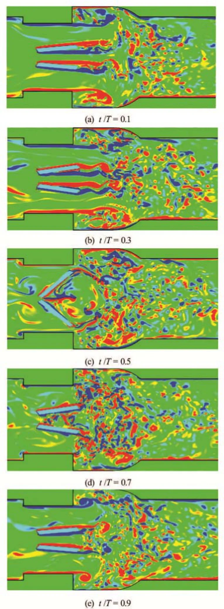
Fig.8 （Color online） Instantaneous flow fields at an -xz plane cutting through the middle of the leaflets: Spanwise vorticity

Fig.9 （Color online） Landslide generated waves. The air-water interface is colored by the elevation

2.4Free-surface hydrodynamics

Numerical simulation of free-surface hydrodynamics is of particular interest in the field of naval architecture and ocean engineering［47］. In Ref.［48］ the waves generated by 3-D sliding masses were studied using both large-scale wave tank experiments and numerical methods. The numerical simulation was performed with an unstructured grid based finite volume approach， in which the free-surface was tracked by a volume-of-fluid method and source terms were introduced in the continuity and momentum equations to represent the presence of the moving solid. Such a treatment is less refined than the velocity interpolation procedures in IBM， but seemed to be acceptable on coarse grids as shown in Ref.［48］. Here the case of a sub-aerial wedge slide as detailed in Ref.［48］ is demonstrated with the motion of the sliding wedge given by laboratory measurement［28］. The snapshots of airwater interface profile are shown in Fig.9. At the beginning， the sliding wedge enters the water slowly and pushes away the water in front of it. As the wedge reaches its full speed， the water around it follows thedownward motion of the wedge and a big cavity appears on top of the wedge. The wedge keeps sinking and water rushes into the cave. A big jet is generated near the shoreline when the left and right flushing waves merge at the centerline. This jet then collapses and strong waves propagate outward. These snapshots qualitatively agree with the simulation in Ref.［48］ very well. The air-water interface fluctuations were compared with the data recorded from a series of wave gauges in the experiment and shown in Ref.［28］ with overall very good agreement.

In Ref.［49］ the air-water turbulent flow past the ship model DTMB 5512 at Fr=0.41 was simulated on a Cartesian grid of 512×512×1024 （2.68×108） points. The smallest grid spacing is about 0.0008L with L the ship length. The instantaneous air-water interface colored by the elevation is shown in Fig.10（a）. The breaking bow waves and scars induced by them are evident. The transom region is very energetic and a lot of wave breaking happens there. Figure 10（b）shows the under-water vortical structures colored by streamwise vorticity. It is remarkable that two vortical filaments induced by bow waves on each side of ship hull retain their sizes and strength and extend into the far wake where the grid becomes very coarse.

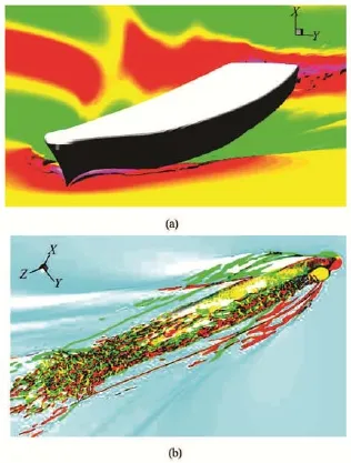
Fig.10 （Color online） Ship model DTMB 5512 at （Fr=0.41）

Some very attractive properties of IBM for the numerical simulation of free-surface hydrodynamics are the ease of case setup， the efficiency of the overall approach， and the accuracy of wave capturing， even on relatively coarse grids， which make the IBM particular suitable for fast prototyping computations in the initial design stage.

3. Concluding remarks

IBM has long been established as a versatile and cost-effective approach for FSIs problems since its introduction. It is very attractive in that a simple forcing term is added to the momentum equation to represent the effect of a complex immersed boundary on the fluid flow， without modifying the regular finite difference schemes on a fixed Cartesian grid. Many variants have been developed for a wide range of applications. In this paper， some development along the line of SIDF approaches has been summarized. Major components involved in simulation algorithms for FSI problems， such as basic fluid flow solvers， immersed boundary setup procedures， treatments of stationary and moving boundaries， and strong coupling schemes，are discussed with comments on their pros and cons. Practical applications from several areas such as particulate flows， flow-induced vibrations， biofluid dynamics， and free-surface hydrodynamics are demonstrated.

To further expand the application regime of SIDF-IBM， a major effort has to be made in the wall modeling techniques for high Reynolds number turbulent flows. Some work has been done using wall functions in the local solution reconstruction near the immersed boundary［50］， but too many assumptions are involved in the derivations of wall functions， which made them inadequate for IBM with highly irregular near-wall point distributions. Local grid refinement techniques， such as block-wise or octree based including adaptive approaches， can greatly enhance the gridding flexibility of IBM， but at a price of more complicated algorithms. On the other hand， mathematical models of more complex physical phenomena can be explored within the IBM framework. One particularly relevant field is the hydroelasticity of ships. Traditional approaches usually involve complicated solver coupling procedures and grid deformation algorithms［51］. Whereas with IBM， instead of treating each other as a black box， the structural solver and the CFD solver can be coupled tightly and efficiently［52-55］. In addition， cavitation is a multi-phase flow phenomenon frequently seen in hydraulic machinery［56］such as pumps， turbines， propellers， etc.. They are characterized by complex geometries with moving components and pose major numerical difficulties to traditional boundaryconforming approaches. Combined with LES methodologies［57］， IBM can be a viable choice for high-fidelity cavitation modeling［58］. As the high performance computing is advancing to the exa-scale era， IBM is expected to embrace many exciting challenges in fluid dynamics simulations.

References

［1］LEONARD A. Computing three-dimensional incompressible flows with vortex elements［J］. Annual Review of Fluid Mechanics， 1985， 17（1）: 523-559.

［2］MONAGHAN J. Smoothed particle hydrodynamics and its diverse applications［J］. Annual Review of Fluid Mechanics， 2012， 44: 323-346.

［3］TUCKER P.， PAN Z. A cartesian cut cell method for incompressible viscous flow［J］. Applied Mathematical Modelling， 2000， 24（8）: 591-606.

［4］INGRAM D. M.， CAUSON D. M. and MINGHAM C. G. Developments in cartesian cut cell methods［J］. Mathematics and Computers in Simulation， 2003， 61（3）: 561-572.

［5］PESKIN C. S. Flow patterns around heart valves: A numerical method［J］. Journal of Computational Physics，1972， 10（2）: 252-271.

［6］PESKIN C. S. Numerical analysis of blood flow in the heart［J］. Journal of Computational Physics， 1977， 25（3）: 220-252.

［7］PESKIN C. S. The immersed boundary method［J］. Acta Numerica， 2002， 11: 479-517.

［8］GOLDSTEIN D.， HANDLER R. and SIROVICH L. Modeling a no-slip flow boundary with an external force field［J］. Journal of Computational Physics， 1993， 105（2）: 354-366.

［9］SAIKI E. M.， BIRINGEN S. Numerical simulation of a cylinder in uniform flow: Application of a virtual boundary method［J］. Journal of Computational Physics， 1996，123（2）: 450-465.

［10］ MOHD-YUSOF J. Combined immersed-boundary/B-spline methods for simulations of flow in complex geometries［R］. Stanford， CA， USA: Annual Research Briefs，Center for Turbulence Research. Stanford University，1997， 317-327.

［11］ FADLUN E. A.， VERZICCO R. and ORLANDI P. et al. Combined immersed-boundary finite-difference methods for three-dimensional complex flow simulations［J］. Journal of Computational Physics， 2000， 161（1）: 35-60.

［12］ KIM J.， KIM D. and CHOI H. An immersed-boundary finite-volume method for simulations of flow in complex geometries［J］. Journal of Computational Physics， 2001，171（1）: 132-150.

［13］ TSENG Y. H.， FERZIGER J. H. A ghost-cell immersed boundary method for flow in complex geometry［J］. Journal of Computational Physics， 2003， 192（2）: 593-623.

［14］ BALARAS E. Modeling complex boundaries using an external force field on fixed cartesian grids in large-eddy simulations［J］. Computers and Fluids， 2004， 33（3）: 375-404.

［15］ UHLMANN M. An immersed boundary method with direct forcing for the simulation of particulate flows［J］. Journal of Computational Physics， 2005， 209（2）: 448-476.

［16］ FENG Z. G.， MICHAELIDES E. E. Proteus: A direct forcing method in the simulations of particulate flows［J］. Journal of Computational Physics， 2005， 202（1）: 20-51.

［17］ ZHANG N.， ZHENG Z. An improved direct-forcing immersed-boundary method for finite difference applications［J］. Journal of Computational Physics， 2007， 221（1）: 250-268.

［18］ VANELLA M.， BALARAS E. A moving-least-squares reconstruction for embedded-boundary formulations［J］. Journal of Computational Physics， 2009， 228（18）: 6617-6628.

［19］ YANG X.， ZHANG X. and LI Z. et al. A smoothing technique for discrete delta functions with application to immersed boundary method in moving boundary simulations［J］. Journal of Computational Physics， 2009，228（20）: 7821-7836.

［20］ PINELLI A.， NAQAVI I. and PIOMELLI U. et al. Immersed-boundary methods for general finite-difference and finite-volume Navier-Stokes solvers［J］. Journal of Computational Physics， 2010， 229（24）: 9073-9091.

［21］ KEMPE T.， FRÖHLICH J. An improved immersed boundary method with direct forcing for the simulation of particle laden flows［J］. Journal of Computational Physics，2012， 231（9）: 3663-3684.

［22］ YANG J.， BALARAS E. An embedded-boundary formulation for large-eddy simulation of turbulent flows interacting with moving boundaries［J］. Journal of Computational Physics， 2006， 215（1）: 12-40.

［23］ BALARAS E.， YANG J. Nonboundary conforming methods for large-eddy simulations of biological flows［J］. Journal of Fluids Engineering， 2005， 127（5）: 851-857.

［24］ YANG J.， PREIDIKMAN S. and BALARAS E. A strongly coupled， embedded-boundary method for fluid-structure interactions of elastically mounted rigid bodies［J］. Journal of Fluids and Structures， 2008， 24（2）: 167-182.

［25］ YANG J.， STERN F. A simple and efficient direct forcing immersed boundary framework for fluid-structure interactions［J］. Journal of Computational Physics， 2012，231（15）: 5029-5061.

［26］ YANG J.， STERN F. Robust and efficient setup procedure for complex triangulations in immersed boundary simulations［J］. Journal of Fluids Engineering， 2014， 135（10）: 101107.

［27］ YANG J.， STERN F. A non-iterative direct forcing immersed boundary method for strongly-coupled fluid-solid interactions［J］. Journal of Computational Physics， 2015，295: 779-804.

［28］ YANG J.， STERN F. Sharp interface immersed-boundary/ level-set method for wave-body interactions［J］. Journal of Computational Physics， 2009， 228（17）: 6590-6616.

［29］ YANG J.， STERN F. Efficient simulation of fully coupled wave-body interactions using a sharp interface immersedboundary/level-set method［C］. Proceedings of ASME 2010 3rd Joint US-European Fluids Engineering Summer Meeting. Montreal， Canada， 2010.

［30］ YANG J.， STERN F. A sharp interface direct forcing immersed boundary approach for fully resolved simulations of particulate flows［J］. Journal of Fluids Engineering，2013， 136（4）: 040904.

［31］ BEDDHU M.， TAYLOR L. K. and WHITFIELD D. L. Strong conservative form of the incompressible Navier-Stokes equations in a rotating frame with a solution procedure［J］. Journal of Computational Physics， 1996，128（2）: 427-437.

［32］ KIM D.， CHOI H. Immersed boundary method for flow around an arbitrarily moving body［J］. Journal of Computational Physics， 2006， 212（2）: 662-680.

［33］ LEONARD B. P. A stable and accurate convective modelling procedure based on quadratic upstream interpolation［J］. Computer Methods in Applied Mechanics and Engineering， 1979， 19（1）: 59-98.

［34］ JIANG G.-S.， SHU C.-W. Efficient implementation of weighted ENO schemes［J］. Journal of Computational Physics， 1996， 126（1）: 202-228.

［35］ BEAM R. M.， WARMING R. F. An implicit finite-difference algorithm for hyperbolic systems in conservationlaw form［J］. Journal of Computational Physics， 1976，22（1）: 87-110.

［36］ MATTOR N.， WILLIAMS T. J. and HEWETT D. W. Algorithm for solving tridiagonal matrix problems in parallel［J］. Parallel Computing， 1995， 21（11）: 1769-1782.

［37］ CHOI H.， MOIN P. Effects of the computational time step on numerical solutions of turbulent flow［J］. Journal of Computational Physics， 1994， 113（1）: 1-4.

［38］ BROWN P. N.， FALGOUT R. D. and JONES J. E. et al. Semicoars ening multigrid on distributed memory machines［J］. SIAM Journal on Scientific Computing， 2000，21（5）: 1823-1834.

［39］ SWARZTRAUBER P. N. A direct method for the discrete solution of separable elliptic equations［J］. SIAM Journal on Numerical Analysis， 1974， 11（6）: 1136-1150.

［40］ POPINET S. The GNU triangulated surface library［OL］. http://gts.sourceforge.net/， ［Online， accessed 1-January-2012］， 2011.

［41］ O'ROURKE J. Computational geometry in C［M］. 2nd Edition， New York， USA: Cambridge University Press，1998.

［42］ IACCARINO G.， VERZICCO R. Immersed boundary technique for turbulent flow simulations［J］. Applied Mechanics Reviews， 2003， 56（3）: 331-347.

［43］ ERICSON C. Real-time collision detection［M］. San Francisco， USA: Morgan Kaufmann Publishers， 2005.

［44］ MORDANT N.， PINTON J. F. Velocity measurement of a settling sphere［J］. European Physical Journal B - Condensed Matter and Complex Systems， 2000， 18（2）: 343-352.

［45］ GLOWINSKI R.， PAN T. and HESLA T. et al. A fictitious domain approach to the direct numerical simulation of incompressible viscous flow past moving rigid bodies: Application to particulate flow［J］. Journal of Computational Physics， 2001， 169（2）: 363-426.

［46］ ANDERSEN A.， PESAVENTO U. and WANG Z. J. Unsteady aerodynamics of fluttering and tumbling plates［J］. Journal of Fluid Mechanics， 2005， 541: 65-90.

［47］ STERN Frederick， WANG Zhao-yuan and YANG Jianming et al. Recent progress in CFD for naval architecture and ocean engineering［J］. Journal of Hydrodynamics，2015， 27（1）: 1-23.

［48］ LIU P. L. F.， WU T. R. and RAICHLEN F. et al. Runup and rundown generated by three-dimensional sliding masses［J］. Journal of Fluid Mechanics， 2005， 536: 107-144.

［49］ YANG J.， BHUSHAN S. and SUH J.， et al. Large-eddy simulation of ship flows with wall-layer models on Cartesian grids［C］. Proceedings of the 27th Symposium on Naval Hydrodynamics， Seoul， Korea， 2008.

［50］ BHUSHAN S.， CARRICA P. M. and YANG J. et al. Scalability studies and large grid computations for surface combatant using CFD Ship-Iowa［J］. International Journal of High Performance Computing Applications （in Press）.

［51］ PAIK K. J.， CARRICA P. M. and LEE D. et al. Strongly coupled fluid-structure interaction method for structural loads on surface ships［J］. Ocean Engineering， 2009，36（17-18）: 1346-1357.

［52］ YU Zhao-sheng， SHAO Xue-ming. A three-dimensional fictitious domain method for the simulation of fluid-structure interactions［J］. Journal of Hydrodynamics， 2010，22（5Suppl.）: 178-183.

［53］ LIAO K.， HU C. A coupled fdm-fem method for free surface flow interaction with thin elastic plate［J］. Journal of Marine Science and Technology， 2013， 18（1）: 1-11.

［54］ SHIN Sangmook， BAE Sung Yong. Simulation of water entry of an elastic wedge using the FDS scheme and HCIB method［J］. Journal of Hydrodynamics， 2013， 25（3）: 450-458.

［55］ TANG Chao， LU Xi-yun. Self-propulsion of a three-dimensional flapping flexible plate［J］. Journal of Hydrodynamics， 2016， 28（1）: 1-9.

［56］ LUO Xian-wu， JI Bin and TSUJIMOTO Yoshinobu. A review of cavitation in hydraulic machinery［J］. Journal of Hydrodynamics， 2016， 28（3）: 335-358.

［57］ BALARAS E.， SCHROEDER S. and POSA A. Largeeddy simulations of submarine propellers［J］. Journal of Ship Research， 2015， 59（4）: 227-237.

［58］ MICHAEL T.， YANG J. and STERN F. Sharp interface cavitation modeling using volume-of-fluid and level set methods［C］. Proceedings of the ASME 2013 Fluids Engineering Summer Meeting. Incline Village， Nevada，USA， 2013， FEDSM2013-16479.

（August 8， 2016， Revised October 12， 2016）

* Biography： Jianming YANG， Male， Ph. D.