HAN Jiang-bo (韩江波)

School of Earth Sciences and Engineering, Hohai University, Nanjing 210098, China

State Key Laboratory of Hydrology-Water Resources and Hydraulic Engineering, Nanjing Hydraulic Research Institute, Nanjing 210029, China, E-mail: han.j.b@163.com

ZHOU Zhi-fang (周志芳)

School of Earth Sciences and Engineering, Hohai University, Nanjing 210098, China

FU Zhi-min (傅志敏)

College of Hydrology and Water Resources, Hohai University, Nanjing 210098, China

WANG Jin-guo (王锦国)

School of Earth Sciences and Engineering, Hohai University, Nanjing 210098, China

Vadose-zone moisture dynamics under radiation boundary conditions during a drying process*

HAN Jiang-bo (韩江波)

School of Earth Sciences and Engineering, Hohai University, Nanjing 210098, China

State Key Laboratory of Hydrology-Water Resources and Hydraulic Engineering, Nanjing Hydraulic Research Institute, Nanjing 210029, China, E-mail: han.j.b@163.com

ZHOU Zhi-fang (周志芳)

School of Earth Sciences and Engineering, Hohai University, Nanjing 210098, China

FU Zhi-min (傅志敏)

College of Hydrology and Water Resources, Hohai University, Nanjing 210098, China

WANG Jin-guo (王锦国)

School of Earth Sciences and Engineering, Hohai University, Nanjing 210098, China

(Received May 29, 2013, Revised November 18, 2013)

In order to better understand the soil moisture dynamics during a drying process, a soil column experiment is conducted in the laboratory, followed by the numerical modeling with consideration of the coupled liquid water, water vapor and heat transport in the vadose zone. Results show that there are three distinct subzones above the water table according to the temporally dynamic variation of the water content profiles. Zone 1 sees a decrease in the water contents in the upper profiles (0 m-0.05 m) due to a negative net water flux in this zone where the upward isothermal water vapor flux becomes the main flow mechanism in the soils. In contrast, the water content within Zone 2 in the depth ranging from 0.05 m to 0.37 m sees an apparent increase over time, resulting from the positive net thermal water-vapor and isothermal liquid-water fluxes into this layer. Zone 3 (0.37 m-0.65 m) also sees an apparent decrease in the water content since the isothermal liquid water flux carries the liquid water either upward out of this region for vaporization or downward to the water table as a recharge to the groundwater.

moisture dynamics, soil water flux, vadose zone, soil column experiment, soil drying

Introduction

The temporal variations of the water content in the shallow vadose zone driven by matric potentials and temperature gradients could induce the soil water fluxes in both gas and liquid phases, especially in semi-arid and arid areas, and could play a key role in the land-atmosphere exchanges. The soil moisture near the land surface controls the partitioning of the precipitation into the quick storm runoff and infiltration and the partitioning of incoming solar and atomspheric energy into the latent and sensible heat fluxes[1]. In addition, the soil water moisture and the temperature have critical influences on many physical processes in the vadose zone, such as the solute transport and the volatilization, the salt accumulation during the soil drying, the nitrogen transformations and transport in the soil-plant system, and the fundamental biological processes such as the microbial activity and the plant growth[2].

Philip and De Vries (henceforth PDV) provided the first theory on the interactions between liquid water, water vapor, and heat transport in the porous medium, and the mathematical model of liquid water and water vapor fluxes in soils driven by both matric potentials and soil temperature gradients[3]. Based on the PDV model, many laboratory and field experiments as well as the numerical modelings were conducted to study the simultaneous heat and water transport inthe unsaturated porous media with complicated boundaries[3,4].

The coupled theory of liquid water, water vapor and heat transport in the unsaturated zone has been validated and modified under numerous laboratory[4-7]and field conditions[2,3,8-10]. However, the measurement techniques and numerical approaches should be improved before the theory can further be advanced. Firstly, the one-dimensional column experiments were often affected by ambient temperature conditions[11], leading to undesired two dimensional distributions of both temperature and water. Secondly, some column experiments were commonly conducted using the destructive sampling method to obtain the soil water content in laboratory, which prevented the measurement of transient conditions and precluded the application of more than one set of boundary conditions to a given soil sample[12]. Thirdly, many laboratory experiments were performed in closed soil columns where there was no water movement into or out of the top boundary, without considering the evaporation or the land-atmospheric boundary conditions[13]. Fourthly, the field experiments typically provided many sets of sparse data to account for the heterogeneous soil and complicated transient boundary conditions, often with results much different than those predicted by the theory[4].

The complete evaluation of the movement of liquid water, water vapor, and heat in the vadose zone can be accomplished by simultaneously solving the system of equations for the surface water and energy balances, subsurface heat transport, and variably saturated flow. These equations need to be solved numerically since they are highly nonlinear and strongly coupled. However, due to insufficient experiment data and the complexity of available codes, most coupled models strongly depend on empirical approaches or simplification of the models by neglecting some transport processes[4]. Although the simplification of models reduced the calculation costs and the divergence probability, the validity may become highly questionable. In particular, many models were validated and calibrated with the steady-state moisture and temperature distributions and /or many optimized parameters[1,14], which faces a harsh criticism for not being adequately under various conditions. Moreover, these methods usually were better applied to a relatively high water content condition than a lower water content during the soil drying[5].

In this study, to better understand the soil water dynamics in the vadose zone during the soil drying, we use an open soil column equipped with a network of soil water and temperature sensors to obtain the continuous moisture and temperature data under the high radiation boundary condition. Because of the complexity of the coupled liquid water, water vapor, and heat transport in the unsaturated zone, the simulation models are then used to gain detailed insights into a variety of water transport mechanisms in the vadose zone. And then the soil water dynamics during the soil drying can be sufficiently evaluated by using the numerical results on temporal variations in the soil water fluxes.

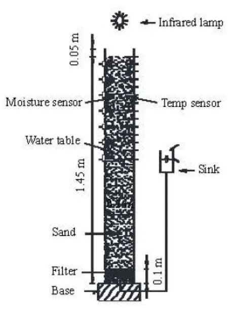
Fig.1 The schematic layout of the soil column and sensors

1. Experimental set-up

In this experiment, the wet sand (with grain sizes from 5×10-5m to 10-3m, and a mean value of about 3.5×10-4m) is uniformly packed in the soil column (0.20 m in diameter by 1.50 m in height, made from polymethyl methacrylate) with a bulk density of 1 620 kg/m3(Fig.1). Through the column walls, 14 temperature and 7 soil moisture sensors are installed radially at the center of the soil column every 0.05 m and 0.10 m, respectively. The water content and temperature data are continuously monitored at the intervals of 5 min, using the dielectric soil moisture sensors (EC-5 Soil Moisture Sensor), and the temperature sensors, respectively. The air relative humidity above the column is measured by using the relative humidity sensor (12-Bit Temp/RH Smart Sensor). Other temperature sensors for monitoring the temperatures in the saturated zone and air are used but not shown in Fig.1. All sensors are connected to the data logger system (HOBO Weather Station-H21-001) for automatic data recording. In order to reduce the ambient temperature interference, the rubber and plastic insulation materials are used to wrap around the lateral sides of the soil column and to produce approximately one-dimensional temperature distributions in soils.

The soil is initially saturated and then drained to reach an equilibrium with a constantly maintained water table at the depth of 0.65 m below the soil surface. The constant water table is maintained through the peristaltic pump outside the column. The upper boundary conditions are the constant radiation main-tained by the infrared lamp (275 W), zero wind speed, and the constant air temperature in the laboratory. The lower boundary conditions are the constant temperature at the water table. The experiment is conducted for 36 h until the water content and temperature data are approximately constant over time.

2. Heat and water transport model

2.1Liquid water and water vapor flow

The general partial differential equation for describing the one-dimensional transient water flow under variably saturated, non-isothermal conditions can be expressed as[7]

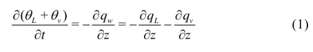
where θLis the volumetric liquid water content, θvis the volumetric water vapor content, θairis the volumetric air content and ρLis the density of the liquid water, qwis the total water flux, qLand qvare the flux densities of the liquid water and the water vapor, t is the time, and z is the spatial coordinate, positive upward.

The PDV model describes the water vapor movement due to both the temperature and the matric potential gradients and the liquid water movement due both to the gravity infiltration and the transport resulting from both the matric potential and the temperature gradients. Thus, the flux density of the liquid water, qL, and the flux density of the water vapor, qvare expressed, as:

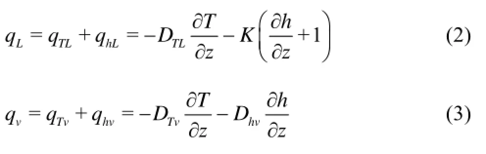
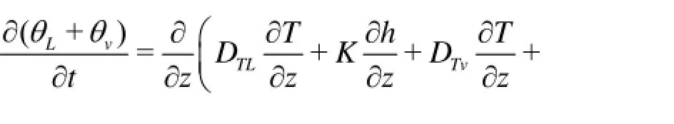
where qTL, qhLare the thermal and isothermal liquid water fluxes, qTv, qhvare the thermal and isothermal water vapor fluxes, T is the soil temperature, h is the pressure head, DTLand K are the thermal and isothermal hydraulic conductivities for the liquid phase fluxes, and DTv, Dhvare the thermal and isothermal hydraulic conductivities for the water vapor fluxes. Combining Eqs.(1) through (3), the governing liquid water and water vapor equation can be expressed as

2.2Soil hydraulic properties

Fayer and Simmons proposed an unsaturated hydraulic property model to better represent the soil water retention curve and the unsaturated hydraulic conductivity at low water contents[5]:

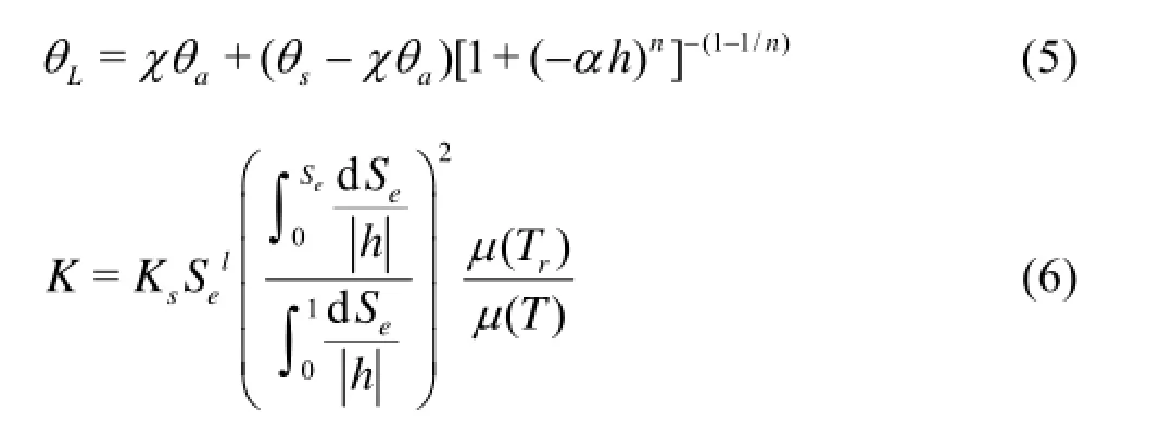
where θsis the saturated water content, α, n and θaare the empirical shape parameters, χ is adsorption of water on soil, where hmis the pressure head when the water content is equal to 0, Ksis the saturated hydraulic conductivity, Seis the effective liquid saturation, l is the pore connectivity coefficient, μ is the dynamic viscosity of the liquid water, which explains the temperature dependence of the unsaturated hydraulic conductivity, and Tris the reference temperature. The soil water retention curves are obtained by measurements in the laboratory. And the Fayer and Simmons model in Eqs.(5) and (6) is fitted with the measurement data, leading to θs=0.335, θa=0.098, α=0.165 m-1, and n=1.49.

The thermal hydraulic conductivity for the liquid flux, DTL, is defined as

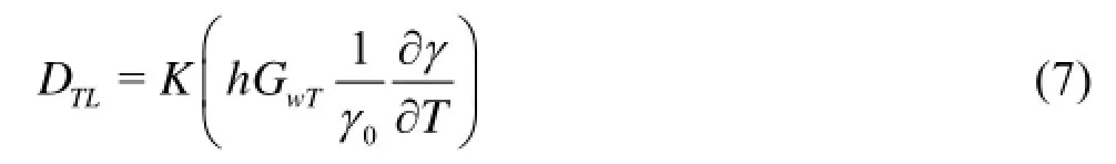
where GwTis the gain factor, which corrects the temperature dependence of the surface tension, γ0, γ are the surface tensions of the soil water at 25oC. The thermal (DTv) and isothermal (Dhv) vapor hydraulic conductivities are described by, respectively:

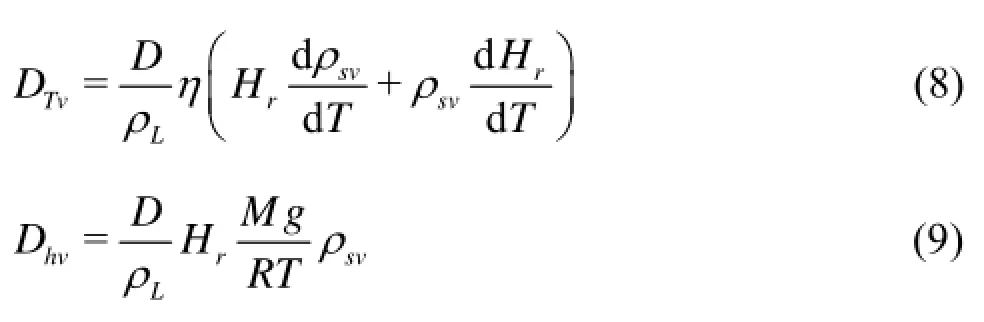
where D is the vapor diffusivity in the soil, η is the enhancement factor, Hris the relative humidity, ρsvis the saturated vapor density at T, M is the mo-lecular weight of water, g is the gravitational acceleration, and R is the universal gas content. The diffusivity of the water vapor D in the soil is described as where Dais the diffusivity of the water vapor in air, Tabsis absolute temperature, and Ω is the tortuosity factor as a function of the air content. The relative humidity, Hr, can be described by using the thermodynamic relationship between the liquid water and the water vapor in the soil pores

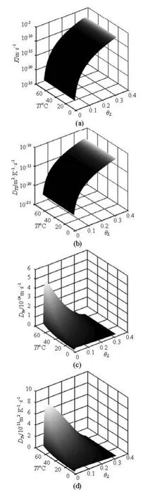
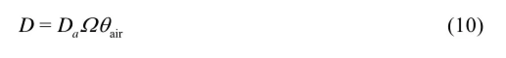
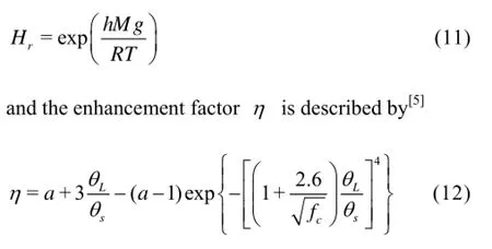
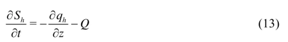
Fig.2 The isothermal liquid, thermal liquid, isothermal vapor and thermal vapor hydraulic conductivities as functions of soil temperatures and water contents

where a is an empirical constant to be determined by data fitting in this study, and fcis the mass fraction of clay.

The soil temperature and water content dependencies of the transport conductivities for the liquid water and the water vapor are shown in Fig.2. K and DTLincrease by orders of magnitude with the increase of the water content, but increase slightly with the increase of the soil temperature, both of which assume similar shapes. DTvand Dhvfirst increase and then decrease within one order of magnitude with the increase of the water content, and increase significantly with the increase of the temperature.

2.3Heat transport and soil thermal properties

The governing equation for the one-dimensional movement of energy in a variably saturated vadose zone is given by

where Shis the storage of heat in the soil, qhis the total soil heat flux density, and Q represents sources and sinks of energy. The storage of the heat Shin the soil is

where Cs, Cwand Cvare the volumetric heat capacities of the dry soil particles, the liquid water and the water vapor, and θnis the volumetric fraction of thesolid phase. The soil heat flux densityhq, accounting for the sensible heat of the conduction, the sensible heat by the convection of the liquid water and the water vapor, and the latent heat by the vapor flow, can be described as

where λ is the apparent soil thermal conductivity described by

where b1, b2and b3are empirical parameters, L0is the volumetric latent heat of vaporization of the water. Combining the continuity equation with Eqs.(14) and (15), we obtain the governing equations for the movement of energy in soils

where Cprepresents the volumetric heat capacity of the moist soil, and the contribution of air to Cpis assumed to be negligible, and the last term on the right hand side of Eq.(17) represents the lateral heat loss, which accounts for the energy flux through the column walls, and hTis the energy transfer coefficient determined by other experiments by using the heat transfer method.

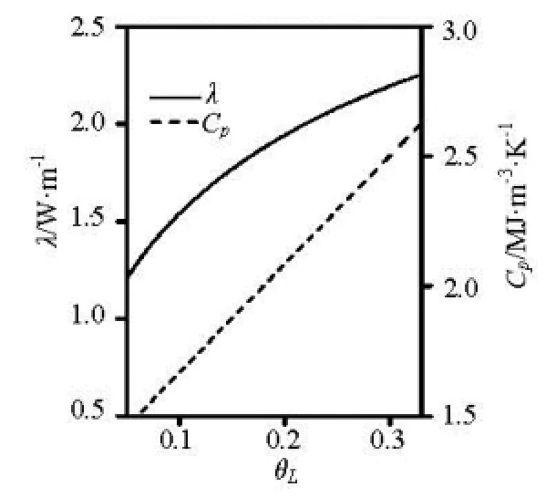
Fig.3 The thermal conductivity and volumetric heat capacity of the moist soil as functions of water contents

λ andpC dependencies of the water content are shown in Fig.3. Cpincreases linearly with the increase of the water content, whereas λ shows a typical nonlinear relation with the water content.

2.4Initial and boundary conditions

The top boundary for the temperature is assigned to a fitted time function of measured temperature valuoes. And the initial soil temperature is observed to be 8C throughout the whole profile. The lowoer boundary temperature at the water table is fixed at 8C since the heat obtained from the soil surface does not reach the location of the water table during the experiment period. The top boundary condition for water can be expressed as

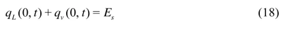
where Esis the surface evaporation rate, calculated from the difference between the water vapor densities of the air, ρva, and the soil surface, ρvs

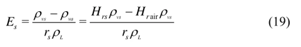
where Hrsand Hrairare the relative humilities at the soil surface and above the column, respectively, and rscan be expressed as[8]

where θrwis an empirical parameter, θtopis the water content in the soil surface layer. The water content at the bottom boundary (0.65 m) of the vadose zone is assumed to be the saturated water content θs.

3. Results and discussions

The governing equations for the liquid water, the water vapor and the heat transport (Eqs.(4) and (17)) combined with the initial and boundary conditions are solved by a commercial software (COMSOL Multiphysics, Version 4.2a) and other codes based on the finite element method in the Matlab Language. The 0.65 m long soil profile is divided into 1 728 elements with a thickness of 3.762×10-5m, and the soil temperatures and the water contents for each discretized node are saved in 100 s intervals. Because the enhancement factor η for the water vapor movement is a parameter described by the empirical relation to explain the disagreement between the observed and calculated data, the parameter a in the enhancement factor in Eq.(12) is chosen as the only parameter to calibrate the model. And the resulting value of a is 2.3.

3.1Temporal and spatial variations in soil temperatures and water contents

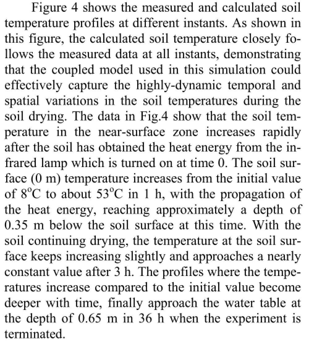
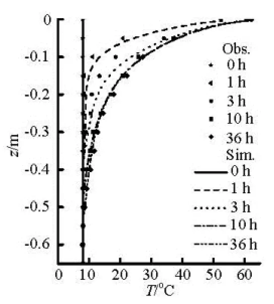
Fig.4 The measured (scatter point) and simulated (solid line) soil temperature profiles at different times

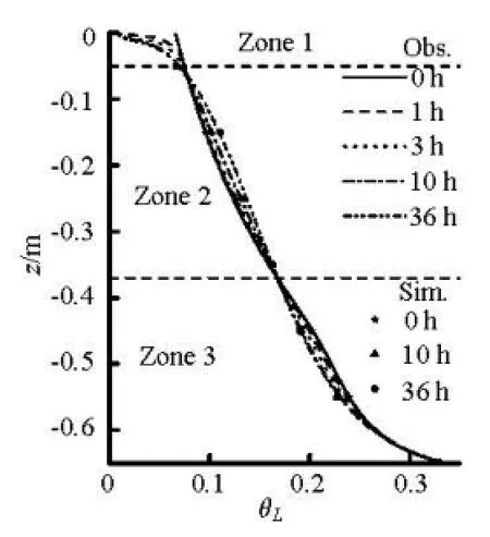
Fig.5 The measured (scatter point) and simulated (solid line) soil water content profiles at different times

It is apparent that the soil temperature profiles between the soil surface and the water table assume clearly concave distributions. This concavity in the temperature profile is resulted from the nonlinear distributions of the soil thermal properties in the vadose zone, i.e., the nonlinear distributions of the soil thermal conductivity and the heat capacity, both of which are functions of the soil water content (Fig.3), typically in non-uniform distributions in the vadose zone (Fig.5). It is also found that the temperature gradient is sharply steeper in the profile, particularly in the upper profiles near the soil surface. The large temperature gradient causes a significant water flow near the soil surface in both the vapor and liquid phases. In the field, this condition usually prevails at warmer seasons of a year in the shallow vadose zone where the soil temperature and the temperature gradients are typically huge.

The water content profiles at different times are shown in Fig.5. The simulated water content also matches well with the measured values in the whole vadose zone at different instants, which shows the validity of the present model in reproducing the moisture dynamics during the soil drying. According to the dynamic variation in the water content profiles, the vadose zone could be divided into three subzones from the top to the bottom, as shown in Fig.5. Zone 1, ranging from the soil surface to the depth of about 0.05 m, shows an expected water loss derived from the soil water evaporation. In contrast, Zone 2, in the depths from 0.05 m to 0.37 m, shows an apparent increase in the water contents over time. And Zone 3 at the depth of about 0.37 m to the water table at the depth of 0.65 m also shows a decrease in the water content profile, resulting from the process of gravity drainage. There are some physical mechanisms behind the highly dynamic water-content profiles in the vadose zone. We will make a detailed analysis about these mechanisms by using numerical results on the evolution of the soil water fluxes in the following section.

3.2Temporal variations in soil water fluxes

After the soil temperature and water content data are obtained from the solutions of the coupled heat and water transport model, the four water-flux components associated with various transport mechanisms, namely, the thermal liquid, the isothermal liquid, the thermal water vapor and the isothermal water vapor fluxes could be discussed. Note that the evolution of the soil water fluxes is closely associated with the dynamics of the water content profiles (Fig.5). Therefore, to get insights of the water content dynamic information during the drying processes, it is necessary to make a detailed analysis of the temporal changes in the four components of the soil water fluxes.

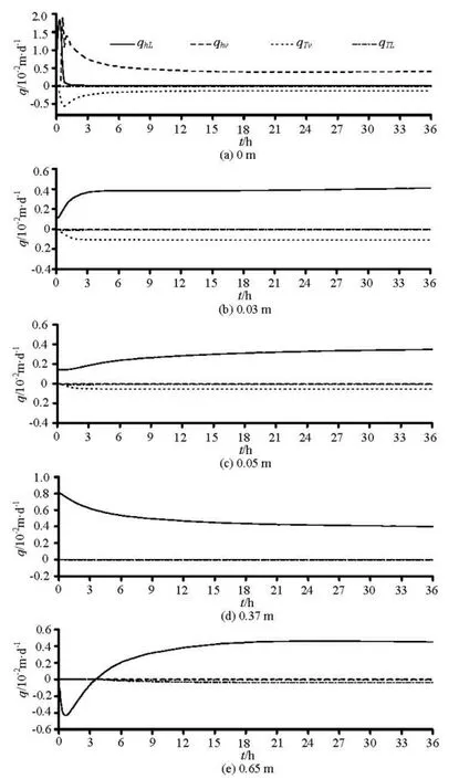
Fig.6 The temporal variations in four components of the soil water flux, namely, thermal liquid, isothermal liquid, thermal water vapor and isothermal water vapor fluxes

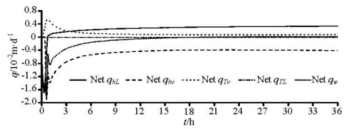
Fig.7 The temporal variations in the net thermal liquid, net isothermal liquid, net thermal water vapor and net isothermal water vapor fluxes as well as the net total water flux within Zone 1

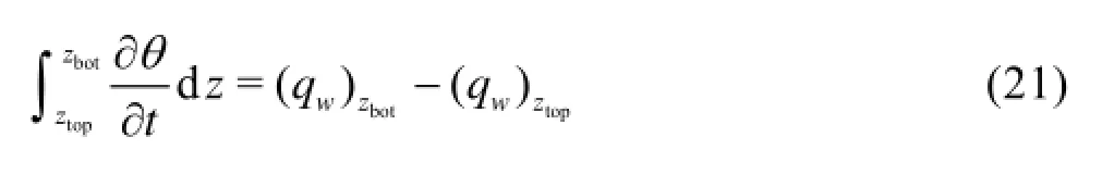
where θ is the total water content, which is approximately equal to the volumetric liquid water content θLbecause the volumetric water vapor content θvaccording to the definition is equal to ρvθair/ρL, is much less than θLby at least five orders of magnitude. zbotand ztopare the bottom and top boundary depths of the three zones. The left-hand side of Eq.(21) represents the net change in the water contents of this zone, whereas the right-hand side is the net water flux into this layer. Thus, the positive net flux into this layer would cause the increase in the water content of this zone, and vice versa.

Figure 7 shows the temporal changes in the net water flux components as well as the net total water flux in Zone 1 (0 m-0.05 m), calculated with Eq.(21). As shown in Fig.7, the net qTvinto Zone 1 is always positive during the 36 h experiment period, suggesting that it would cause an increase in the water storage of Zone 1. In fact, this part of the water vapor as qTvcomes from the upper layer, and would be changed to the liquid water when it comes across the cooler layer than the soil surface where the relative humidity approaches the saturation value. And this part of the liquid water from the condensation of the water vapor would be contributed to the water storage of Zone 1 and partly replenishes the loss of water due to evaporation. The net qhLhas negative values before 0.5 h resulting from the rapid water loss by evaporation at the early period of drying, then increases rapidly and eventually keeps a positive and nearly constant value of 0.0033 m/d at the later period. This positive value for the net qhLat the most time, is clearly due to the relative significant magnitude of qhLat the depths 0 m to 0.05 m (Figs.6(a) to 6(c)), indicating that it would generally contribute to the water storage within the depths of 0 m to 0.05 m, except for the period before 0.5 h when it plays a role in reducing the water storage in this region. In contrast, the net qhvwithin Zone 1 is always negative and has a larger magnitude than other net water-flux components in the whole experiment period. This is the cause why the net total water flux qwis also negative over the experiment period, which eventually leads to a decrease in the water contents of this zone (Fig.5). After 13 h the net total water flux is close to zero because the net qhvand qhLboth have nearly the same magnitudes but in opposite directions during the later period. Thus, after 13 h, the water content in Zone 1 does not decrease anymore, indicating that the system may reach a nearly steady-state condition.

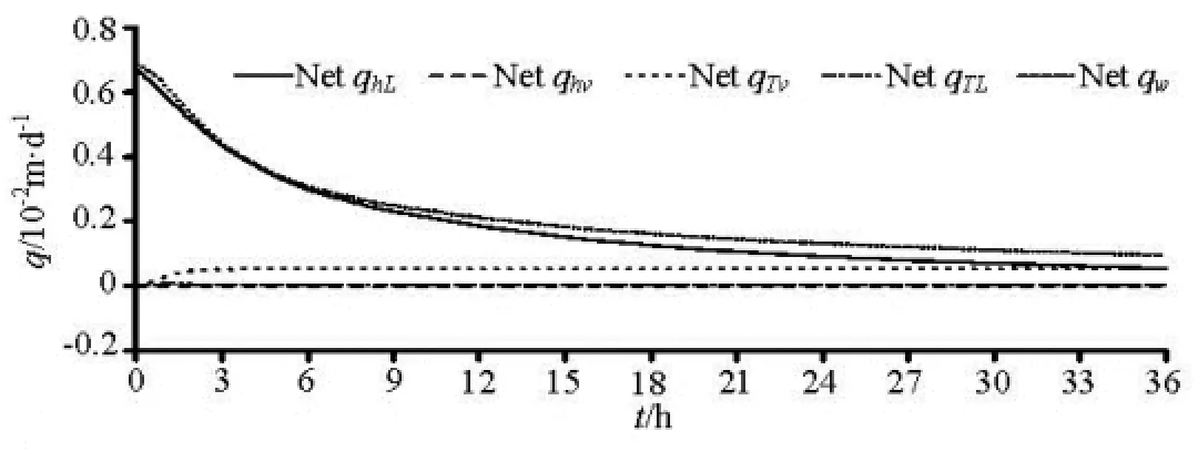
Fig.8 Same as Fig.7 but for Zone 2

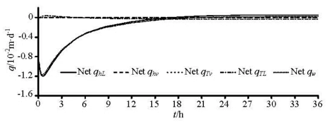
Fig.9 Same as Fig.7 but for Zone 3

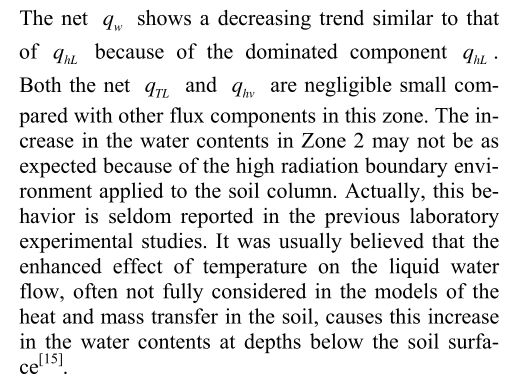
At the depth 0.37 m within Zone 2, qhLbecomes the more dominant mechanism for the water movement as compared to other water flux components which are negligibly small (Fig.6(d)). This suggests that in this zone the matric potential gradient also has a greater influence on the water movement as compared with the effect of the temperature gradient. qhLat the depth of 0.37 m sees a significant decrease at the early time and then gradually approaches a constant value of 0.0040 m/d during the later period. The temporal variation in the net water fluxes into Zone 2 according to Eq.(21) is depicted in Fig.8, as obtained from the differences between the fluxes at depths of 0.05 and 0.37 m. Actually, the calculation from the difference between the fluxes at the boundaries of these three zones is dependent partly on the dividing locations of these three zones. However, a possibly little change in the locations of the boundaries of these three zones would not reverse the trend and shape of the net fluxes shown in Figs.7 through 9. Therefore, it may be assumed that the results presented in these figures are accurate enough to assess the dynamic pattern of the water flux. As shown in Fig.8, the net qhLand qTvand the net total water flux qwall have positive values, which explains the reason for the increase in the water contents within Zone 2 (Fig.5). The net qhLsees a decrease trend in magnitude with time, indicating that the extent of contribution of qhLto the water storage decreases over time, while the contribution from the net qTvsees a slight increase with a relatively smaller magnitude compared with the net qhL

At the depth of 0.65 m (Fig.6(e)) qhLsees a decrease first and then increases over time for about 18 h. Before about 3 h, qhLat the depth of 0.65 m is in downward (negative) direction, indicating that some liquid water moves toward the water table from the upper depths as a groundwater recharge. That is because the effect of the downward gravity on the liquid-water movement is more pronounced than the upward matric potential gradient around the water table during this period. The closer to the water table, the larger the value of K as a function of the water contents will be according to Fig.2 (top left), which could result in a larger qhL. There is an apparent thermal liquid water flux qTLat the depth 0.65 m after approximately 4 h when the heat propagates into this layer from the upper layer (Fig.4). qTLtypically comes into effect where there is a large temperature gradient and high values of DTLformed at the region with high water contents according to Fig.2 (top right). Figure 9 illustrates the temporal variation of the net water fluxes into Zone 3. As shown in Fig.9, the shape of the net total water flux qwclosely follows the net qhL, which suggests that qhLdominates in qwat this layer in the whole experiment period. The big negative net qwat the most time suggests that more water flows out of this zone, eventually resulting in the decrease in the water content in this zone (Fig.5). The magnitude of the net qwis close to zero at the later period of this experiment, indicating that the water storage at this layer would keep nearly constant and does not decrease with time.

Note that at the later period of the experiment, the four components of the total water flux (Fig.6) and the net water fluxes (Figs.7 to 9) all take relatively constant values, which indicates that the system between the soil column and the atmosphere reaches a dynamic balance under the constant water table condition. Then the temperature and the water content at the whole profile could not change with time any more, and the rate of soil drying is also restricted by the constant water supply from the water table.

4. Conclusion

In order to obtain a better understanding of the soil water dynamics in the vadose zone during the soil drying process, an open soil column experiment is conducted under high radiation boundary conditions in the laboratory. The numerical models of the coupled liquid water, water vapor and heat transport, well calibrated by the measured data, are used to simulate the soil water movement with various mechanisms. Results show that there are three subzones in the vadose zone profile during the soil drying according to the temporal dynamics of the soil water content profiles. Zone 1 at the upper profile sees a decrease in the water contents mainly because of qhv, which dominates the total water flux, and has a negative net flux out of this layer due to the soil water evaporation. In contrast, the water content profiles within Zone 2 at the depths from 0.05 m to 0.37 m show an unexpected increase in magnitudes, resulting from the net small qTyand large qhLinto this layer. Zone 3 also sees a decrease in the water contents, mainly due to the decrease in the net qhLat this zone over time. And the effect of the temperature on the water vapor movement can be seen mainly within Zone 1 and Zone 2, and that on the liquid water movement can mainly be seen within Zone 3.

[1] DEB S. K., SHUKLA M. K. and MEXAL J. G. Numerical modeling of water fluxes in the root zone of a mature pecan orchard[J]. Soil Science Society of America Journal, 2011, 75(5): 1667-1680.

[2] GRIFOLL J., GAST J. M. and COHEN Y. Non-isothermal soil water transport and evaporation[J]. Advances in Water Resources, 2005, 28(11): 1254-1266.

[3] SAITO H., SIMUNEK J. and MOHANTY B. P. Numerical analysis of coupled water, vapor, and heat transport in the vadose zone[J]. Vadose Zone Journal, 2006, 5(2): 784-800.

[4] SMITS K. M., CIHAN A. and SAKAKI T. et al. Evaporation from soils under thermal boundary conditions: Experimental and modeling investigation to compare equilibrium and nonequilibrium based approaches[J]. Water Resources Research, 2011, 47(5): W05540.

[5] SAKAI M., TORIDE N. and SIMUNEK J. Water and vapor movement with condensation and evaporation in a sandy column[J]. Soil Science Society of America Journal, 2009, 73(3): 707-717.

[6] GRAN M., CARRERA J. and OLIVELLA S. et al. Modeling evaporation processes in a saline soil from saturation to oven dry conditions[J]. Hydrology and Earth System Sciences, 2011, 15(7): 2077-2089.

[7] SAKAI M., JONES S. B. and TULLER M. Numerical evaluation of subsurface soil water evaporation derived from sensible heat balance[J]. Water Resources Research, 2011, 47(2): W02547.

[8] BITTELLI M., VENTURA F. and CAMPBELL G. S. et al. Coupling of heat, water vapor, and liquid water fluxes to compute evaporation in bare soils[J]. Journal of Hydrology, 2008, 362(3-4): 191-205.

[9] NOVAK M. D. Dynamics of the near-surface evaporation zone and corresponding effects on the surface energy balance of a drying bare soil[J]. Agricultural and Forest Meteorology, 2010, 150(10): 1358-1365.

[10] XIANG L., YU Z. and CHEN L. et al. Evaluating coupled water, vapor, and heat flows and their influence on moisture dynamics in arid regions[J]. Journal of Hydrologic Engineering, 2012, 17(4): 565-577.

[11] HEITMAN J. L., HORTON R. and REN T. et al. An improved approach for measurement of coupled heat and water transfer in soil cells[J]. Soil Science Society of America Journal, 2007, 71(3): 872-880.

[12] HEITMAN J. L., HORTON R. and REN T. et al. A test of coupled soil heat and water transfer prediction under transient boundary temperatures[J]. Soil Science Society of America Journal, 2008, 72(5): 1197-1207.

[13] BACHMANN J., Van DER PLOEG R. R. and HORTON R. Isothermal and nonisothermal evaporation from four sandy soils of different water repellency[J]. Soil Science Society of America Journal, 2001, 65(6): 1599-1607.

[14] DEB S. K., SHUKLA M. K. and SHARMA P. et al. Coupled liquid water, water vapor, and heat transport simulations in an unsaturated zone of a sandy loam field[J]. Soil Science, 2011, 176(8): 387-398.

[15] ASSOULINE S., NARKIS K. and TYLER S. W. et al. On the diurnal soil water content dynamics during evaporation using dielectric methods[J]. Vadose Zone Journal, 2010, 9(3): 709-718.

10.1016/S1001-6058(14)60082-2

* Project supported by the National Natural Science Foundation of China (Grant Nos. 41172204, 41102144), and the Natural Science Foundation of Jiangsu Province of China (Grant Nos. BK2011110, BK2012814).

Biography: HAN Jiang-bo (1981-), Male, Ph. D.

ZHOU Zhi-fang,

E-mail: zhouzf@hhu.edu.cn