Hsinchen Yu(于心澄) Dong Bai(柏栋) Peishan He(何佩珊)Xiaoping Zhang(张小平) Zhongzhou Ren(任中洲) and Qiang Zheng(郑强)

1State Key Laboratory of Lunar and Planetary Sciences,Macau University of Science and Technology,Macau 999078,China

2CNSA Macau Center for Space Exploration and Science,Macau,China

3Department of Physics,Nanjing University,Nanjing 210008,China

4School of Physics Science and Engineering,Tongji University,Shanghai 200092,China

5Key Laboratory of Advanced Micro-Structure Materials(MOE),Tongji University,Shanghai 200092,China

6School of Physical Science and Technology,Tiangong University,Tianjin 300387,China

Keywords: quantum chaos,dynamical localization,resonance and topology

1. Introduction

The quantum kicked rotor (QKR) model is a prototypical model in the quantum chaos area.[1–15]The QKR has been realized by many successful experiments.[13,16–27]Based on the original QKR model, the Maryland model was firstly introduced in the 1980s.[4–7]In the Maryland model, the mass termmequals zero, and the free Hamiltonian of the rotor is proportional to the angular momentum. Although the Maryland model has been studied since the 1980s,previous studies focused on the periodically kicked Maryland model. Those studies considered the original Maryland model,[4–7]noise influences,[28–35]dissipation,[35–38]nonlinearity,[39–47]superballistic transportation[48]and many-body localization.[49]

In 1982, Fishman, Grempel, and Prange[2]firstly found the relationship between the dynamical evolution of the original Maryland model over time and the static electron problem in the one-dimensional (1D) tight-binding lattice. However,the non-periodically kicked Maryland model is hard to be related to the periodic lattices in nature.So,the non-periodically kicked Maryland model failed to raise people’s attention. Due to the optical lattice studied and applied in the area of the quantum simulation and the cold atom, the artificial lattice is realized in the optical lattice.[50–54]By operating the particular magnetic field on the spin-1/2 particle and controlling the pulsed optical lattice, the realization of the non-periodically kicked Maryland model is possible in the optical lattice system.

In the original Maryland model, the periodic evolution of the angular momentum spread appears with irrationalα.Compared to the other cases of the QRKR,the massless case of the QRKR (Maryland model) shows the pattern of the periodic evolution.[48]In this paper, we aim to check whether the periodic kicks raise the periodic evolution in the Maryland model. Therefore,the linearly delayed quantum relativistic Maryland model (LDQRMM), a non-periodically kicked Maryland model, is studied. In the LDQRMM, the kicking potential is not uniform but linearly delayed over time.

In our previous work,[55]the angular momentum spread of the LDQRMM has been found to have the “stable–jump–stable–jump” pattern. The expectation value of ˆp2increases or decreases significantly after a particular number of kicks are performed on the rotor. If the“stable–jump–stable–jump”condition is not satisfied, the angular momentum spread will vibrate until the next “stable–jump–stable–jump” condition is satisfied. Although the “stable–jump–stable–jump” pattern explains the local periodic jumps of the LDQRMM, the long-time transportation characteristics of the angular momentum spread can not be explained by the“stable–jump–stable–jump”pattern.Due to the intrinsic characteristics of long-term transportation in the LDQRMM,our objective in this paper is to interpret the long-term transportation characteristics in the LDQRMM.This work can help one understand the evolution of the angular momentum spread in a non-periodically kicked Maryland model,particularly in the LDQRMM.

The framework of this paper is listed below. In Section 2, a non-periodically kicked Maryland model is introduced as the LDQRMM. The spread of the angular momentum in the LDQRMM is found to be related to the evolution of the characteristic sumS(n) withnin the complex number space. In Section 3, the linearly delayed classical Maryland model(LDCMM)is introduced. We calculate the ensemble average of the angular momentum of the LDCMM. We find that the evolution of the ensemble average of the angular momentum in LDCMM is also related to the characteristic sum. In Section 4, the numerical results of the LDQRMM and LDCMM are shown, respectively. In Section 5, different evolution modes of the characteristic sumS(n) are classified and analyzed with different system parameters,αqandd. In Section 6,we devise experiment proposals to realize the LDQRMM with the optical lattice technology. We discuss the corresponding relationship between the LDQRMM and a spin-1/2 particle in an external magnetic field pulsed 1D lattice. In Section 7,our work in this paper is briefly concluded.

2. Linearly delayed quantum relativistic Maryland model

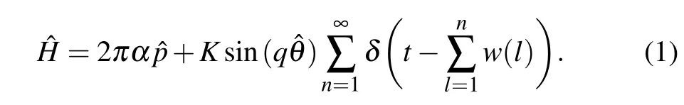
In this section,we introduce the linearly delayed quantum relativistic Maryland model (LDQRMM). In the LDQRMM,the kicking potential is not uniform but linearly delayed over time. The Hamiltonian operator of the LDQRMM reads It is the Hamiltonian operator of a 1D free Dirac rotor kicked by aδ-function potential sequence. 2παis the effective speed of light. The kicking potential is a linearly delayed sequence over time.qis a parameter that determines the period of the function sin in the angular coordinate.w(l)is the internal time between thel-th and(l+1)-th kick,which is linearly delayed as the time of kicks,l,increases,that is,w(l)=1+(l −1)/d.In the LDQRMM, the free Hamiltonian of the LDQRMM is massless. ˆpis the dimensionless angular momentum operator which reads as ˆp=−i∂/∂θ. The parameterK=kTR/¯h,

whereRis the radius of the 1D ring,kis the kick strength of the kicking potential,andTis the unit of time.

In the LDQRMM,the evolution of the kicked rotor is related to the propagator operator ˆF(n), wherenis the time of kicks. The propagator operator ˆF(n)following the(n −1)-th kick in the LDQRMM reads

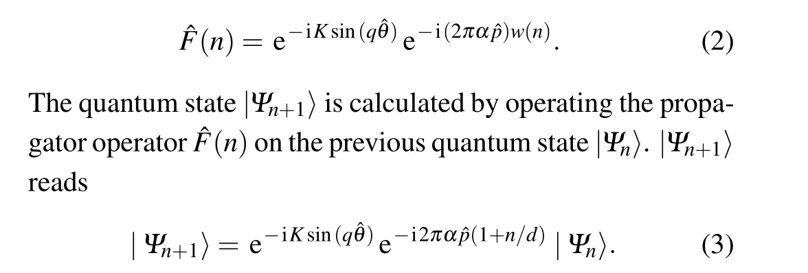
In the angle coordinate representation, the wave function following then-th kick readsΨn+1(θ).Ψn+1(θ)is given by operating the bar of the ˆθcoordinate eigenstate〈θ|on the quantum state|Ψn+1〉,

To study the dynamical evolution characteristic of the LDQRMM,we calculate the angular momentum spread based on the expression of the wave function in Eq.(5). The angular momentum spread ofΨn(θ)is calculated below:

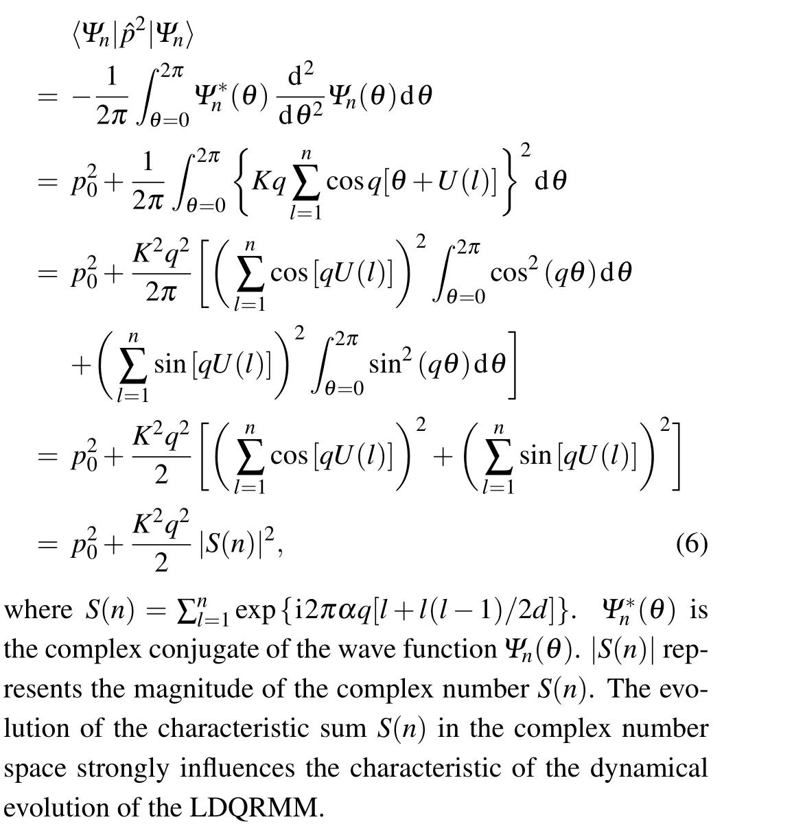
Based on Eq. (6), the characteristic sum directly reflects the resonance and antiresonance characteristic of the angular momentum spread of the corresponding LDQRMM system.The algebraic analysis of the characteristic sum with parameternwill be the key point to understanding the corresponding physical picture of the angular momentum spread.

3. Linearly delayed classical Maryland model

In this section,we introduce the LDCMM.The LDCMM is a classical model that corresponds to the LDQRMM that we have introduced in the above section. The Hamiltonian of the LDCMM reads

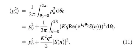
whereθnandpnare the angle coordinate and angular momenta of the LDCMM following thenth kick,respectively. The initial angle coordinate and angular momenta areθ0andp0. According to Eq.(8),

Re(eiqθ0S(n)) represents the real number component of the complex number eiqθ0S(n). According to Eq. (10), it is obvious that the variation in the angular momentum after then-th kick is proportional to the real number component of eiqθ0S(n).

To study the quantum-classical correspondence between the LDQRMM and the LDCMM, we select a special kicked rotor ensemble in the LDCMM, which corresponds to a pure angular momentum eigenstate in the LDQRMM.The ensemble of the LDCMM consists of kicked rotors with the same value of the initial angular momentum 0, but different initial angular coordinatesθ0randomly taken from 0 to 2π.The average angular momentum spread of this ensemble after then-th kick reads Compared with Eq. (6) in the LDQRMM, the spread of the angular momentum in the LDQRMM and its corresponding classical model(LDCMM)is the same. The evolutions of the angular momentum of the LDQRMM and the corresponding LDCMM are all principally influenced by the mathematical properties of the characteristic sumS(n)in the complex number space.

4. Numerical simulations and results

In Sections 2 and 3, we have discussed the evolution of angular momentum in the LDQRMM and LDCMM.This section calculates some results of the average angular momentum spread of the kicked rotors in the LDQRMM and LDCMM.The numerical simulations in this section are based on the equations and discussions in Sections 2 and 3.

4.1. Classical dynamics

The standard map of the LDCMM has been shown in Eq. (9). The results of the LDCMM are based on Eq. (9).In this subsection,we discuss the numerical results of the LDCMM.

In Fig.1,we select three representative cases to compare and discuss the LDCMM trajectories with different system parameters. The initial angular coordinate and the angular momentum of the rotors that we select in Fig.1 areπand 0, respectively. In panels (a)–(c), several discrete “levels” of the angular momentum emerge on a single trajectory. The evolution trajectories of the angular momentum and angular coordinate oscillate at those“levels”or jump between those“levels”. It is called the“stable–jump–stable–jump”pattern.[55]In panel (b), one notices that the evolutionary trajectory is dramatically different from those in panels(a)and(c). The total number of angular momentum“levels”in panel(b)is infinite.Therefore,the evolution of angular momentum at these levels is unbounded in phase space. The ensemble average of the angular momentum is bounded in panel (b). It is consistent with the discussion of the resonance modes of the characteristic sumS(n) in Section 5. However, the angular momentum values periodically jump between the two levels of angular momentum in panel (a). The ensemble average of the angular momentum spreads is localized. In panel (c), the single trajectory is similar to the single trajectory in panel(a). However,the angular momentum levels in panel(c)are not strictly axisymmetric along a particular axis, like those in panel (a).The reason is that the corresponding evolution modes in panels(a)and(c)belong to different classes of homeomorphisms.However, all of them belong to the antiresonance mode. So although their trajectories are bounded and closed, panels(a)and (c) show some differences. In the next section, we will explain those differences by analyzing the characteristic sum.

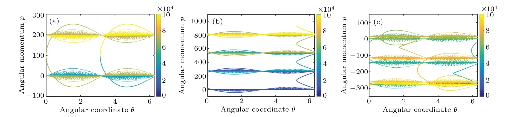
Fig.1. The revolution trajectories of the angular coordinate and the angular momentum in the phase space. The initial angular coordinate and the angular momentum are π and 0,respectively. In panel(a),the system parameters are α =2/3,d=20000,q=1,and K=1.6. In panel(b),d=20002. In panel(c),d=20000/3. The other parameters in panels(b)–(c)are the same as those in panel(a). The x-axis is the angular coordinate. The y-axis is the angular momentum. The colors of the evolution track represent the kicking time. The maximum kicking time is 105. The angular momentum and the angular coordinate are shown in a dimensionless unit.

4.2. Quantum dynamics

In the LDQRMM, the evolution of the wave function is calculated by operating the Floquet operator on the wave function. The Floquet operator of the LDQRMM is given in Eq. (2), which can be separated into a free Hamiltonian propagator operator exp[−i(2παˆp+Mσz)w(n)] and a kicking propagator operator exp[−iKsin(qˆθ)]. The numerical calculations separate a single kick into three steps. Firstly,the discrete Fourier transformation is operated on the initial wave function of the rotor to switch the wave function to the angular momentum representation. The next step is to operate the free Hamiltonian propagator operator on the wave function in the angular momentum representation. In this step, the ˆpoperator is substituted for the eigenvalues. Finally,we perform the inverse Fourier transformation to switch it back to the angular coordinate representation and operate the“δ-function”potential propagator operator on it. Through these three steps, the operation of a single kicking process is performed on the rotor.

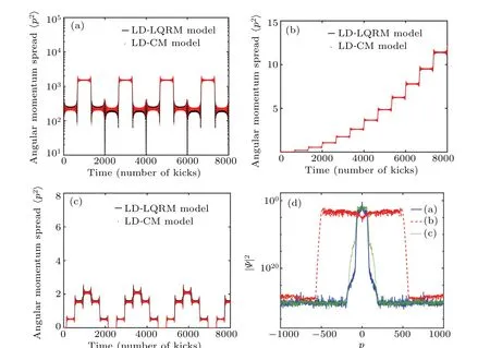
Fig. 2. Panels (a)–(c) show the angular momentum spread 〈p2〉 with different linearly delayed increases. Panel (d) shows the probability density distributions of the cases in panels (a)–(c) after the 8000th kick. In panel (a), d equals to 2000. In panel (b), d =2001. The other parameters are listed below. K=1.6,α =3,and q=1. In panel(c),α =5/3,K=1.6,q=1,and d=2000/3. In panels(a)–(c),the solid black lines show the ensemble average of the angular momentum of the LDQRMM,and the solid red lines are the results of the LDCMM.The angular momentum spread shown is in a dimensionless unit.

In the previous subsection,we study the classical dynamical characteristics of the LDCMM through the simulations of the trajectories of the kicked rotors in the phase space. In the LDCMM, the trajectories of the angular momentum and coordinates are related to the ensemble average of the angular momentum spread. The angular momentum spread of the LDQRMM and LDCMM are calculated in Sections 2 and 3,respectively. The comparison indicates the quantum–classical correspondence between the LDQRMM and LDCMM. In this subsection, the average angular momentum spread in the LDQRMM and LDCMM will be exhibited. The numerical results in Fig.2 are consistent with the analytical discussions in Sections 2 and 3.

The numerical results of the LDQRMM and LDCMM are exhibited in Fig.2. In our numerical calculation,the LDCMM ensemble consists of 103kicked rotors.The initial coordinates of these kicked rotors in the phase space are(θ0,p0). The initial angular coordinateθ0is a random number taken from the values ranging from 0 to 2π. The initial angular momentump0is set as 0. The initial quantum state of the LDQRMM is the angular momentum eigenvector with the eigenvalue 0.The antiresonance condition has been discussed in Section 5.d/gcd{αq,d}∈E is satisfied in panel(a)of Fig.2. The evolution of the angular momentum spread is periodic. Whend=2001,d/gcd{αq,d}∈O. The increase of the angular momentum spread is quadratic in panel (b). Panel (c) shows the evolution of the spread of the angular momentum in the antiresonance case with fractional system parameters.

The numerical results of the angular momentum spread in the LDCMM and the LDQRMM do not show a significant difference. The spread of the angular momentum of the kicked rotors in the LDQRMM and LDCMM is consistent with the convergence property of the characteristic sumS(n) in the complex number space.

5. Classifications and discussion

Based on the discussions in Sections 2 and 3, we have known that the characteristic sumS(n)strongly dominates the spread of the angular momentum in the LDQRMM and LDCMM. Therefore, the analysis of the characteristic sumS(n)in the complex number space is necessary for understanding the evolution characteristics of the angular momentum spread in the LDQRMM and LDCMM. In this section, we discuss the classification of the characteristic sumS(n). This classification is based on the resonance and antiresonance characteristics of the characteristic sum with different parameters.In Subsection 5.1, the characteristic sum evolution with the integer system parameters (αqandd) will be discussed. In Subsection 5.2, a special antiresonance mode of the characteristic sumS(n) with fractional values ofαqanddwill be discussed. We argue that a topological difference exists between the antiresonance modes introduced in the subsections.We will discuss them in the following subsections.

5.1. Resonance and antiresonance modes with integer number parameters

The values of the characteristic sumS(n) with different system parameters are shown in Figs.3 and 4,respectively. In Fig.3, the characteristic sumS(n)periodically evolves in the complex number space asnincreases. However, the magnitude of the characteristic sum (|S(n)|)is linearly divergent as the variablenincreases in Fig.4. The evolution of the characteristic sum in the complex number space shows a significant difference.

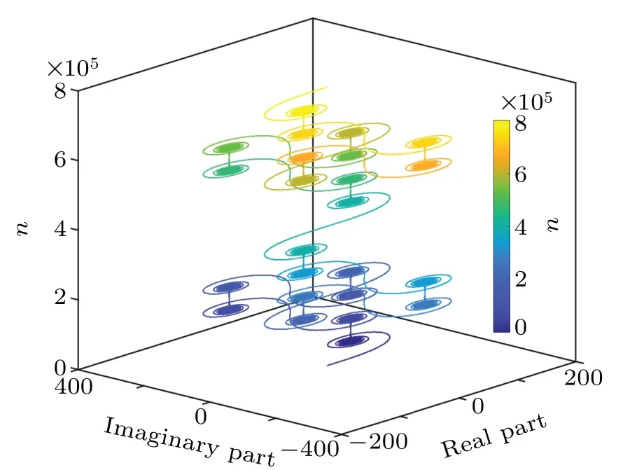
Fig.3.The characteristic sum S(n)with α=3,q=1,and d=20000 in the complex number space.The colors represent n,corresponding to the number of terms to be summed in the calculation of the characteristic sum S(n).

In Fig. 3,S(n)evolves along the same trajectory and returns to the original position in the complex number space.Based on Fig.3,this antisymmetry of the characteristic sum is deduced in Eq.(12). We consider the characteristic sumS(n)having this antisymmetry whennis equal to a number betweenkandk+u.tis an integer number betweenkandk+u. The antisymmetry of the characteristic sum reads

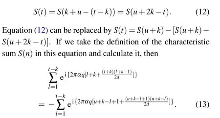
Whenαqanddare integer numbers, we simplify the above equation and get the following result:

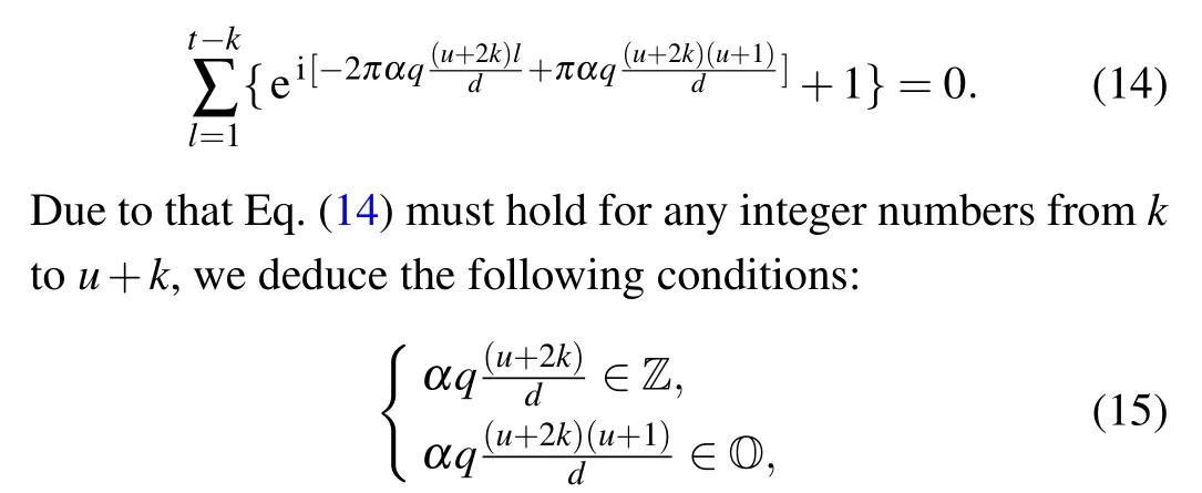
where Z and O represent the set of integers and odd numbers, respectively. According to Eq. (15), we know thatαq(u+2k)/d ∈Z andαq(u+2k)(u+1)/d ∈O. Therefore,u+1∈O. Becauseu+1∈O,we deduce thatu+2k ∈E. Becauseαq(u+2k)/d ∈O in Eq. (15),d/gcd{αq,d}∈E. In a word, the antisymmetric structure of the characteristic sum appears when

E is the set of the even numbers. gcd{αq,d}is the largest common divisor ofαqandd. Under this condition,the angular momentum evolution of the corresponding LDQRMM and LDCMM is periodic in time. Equation (16) is the condition of the antiresonance mode of the characteristic sumS(n)with integer parametersαqandd.

For the resonance mode of the characteristic sum with integer parameters, the evolution ofS(n) is unbounded in the complex number space asnincreases. Based on the characteristic of the characteristic sum shown in Fig. 4, the geometric symmetry in the complex number space is concluded as

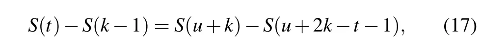
wheretis an integer number betweenkandu+k.kandu+kare arbitrary integers. We take the definition of the characteristic sumS(n)into it and then get the following equation:

Because Eq. (19) must be satisfied for all integers ranging fromktou+k,and exp{i[2παql(l −1)/2d]}is a complex number that is not zero. The resonance condition is deduced as

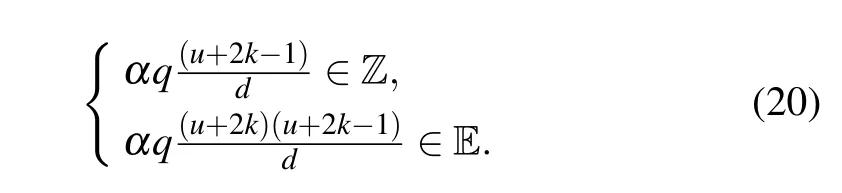
We discuss the conditions in Eq.(20)with two possible cases.In the first case, we suppose thatuis an even number. Sou+2k −1∈O andαq(u+2k −1)/d ∈Z. Therefore, we deduced/gcd{αq,d} ∈O. In the second case,uis supposed to be an odd number. Sou+2k ∈O. According to

αq(u+2k)(u+2k −1)/d ∈E andαq(u+2k −1)/d ∈Z,αq(u+2k −1)/d ∈E. Ifd/gcd{αq,d}∈E, thenαq(u+2k −1)/d ∈O. This result contracts with Eq. (20). Sod/gcd{αq,d}must∈O. Based on the above discussions,the antiresonance condition reads

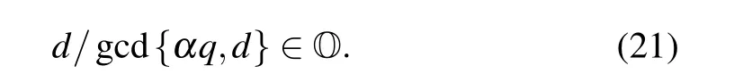
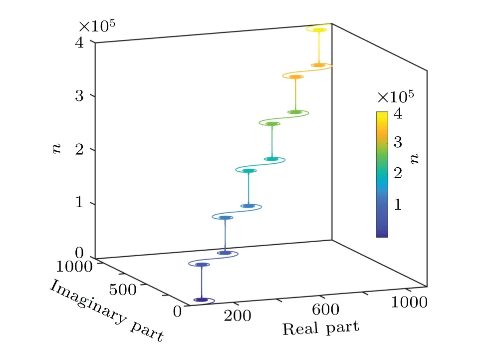
Fig.4. The characteristic sum S(n)with α =3,q=1,and d=20001.The colors represent n, corresponding to the number of terms to be summed in the calculation of the characteristic sum S(n).

In this section, we have considered all cases of the characteristic sum with integer parametersαqandd. Thed/gcd{αq,d}is odd or even determines the resonance or antiresonance properties of the characteristic sumS(n) in the complex number space.

5.2. Antiresonance mode with fractional number parameters

In the above subsections, we have discussed the resonance and antiresonance modes of the characteristic sumS(n)with different integer parameters. In this subsection, we will discuss an antiresonance mode with fractional number parameters. In Fig.5,we plot the evolution of the characteristic sum with this antiresonance mode. In Fig.5,the characteristic sumS(n) shows the rotational symmetry. The characteristic sum evolution is periodic,S(n)=S(n+uT), whereTis the least period to let the whole image invariant under a rotation operation.uis the order of the rotational symmetry.

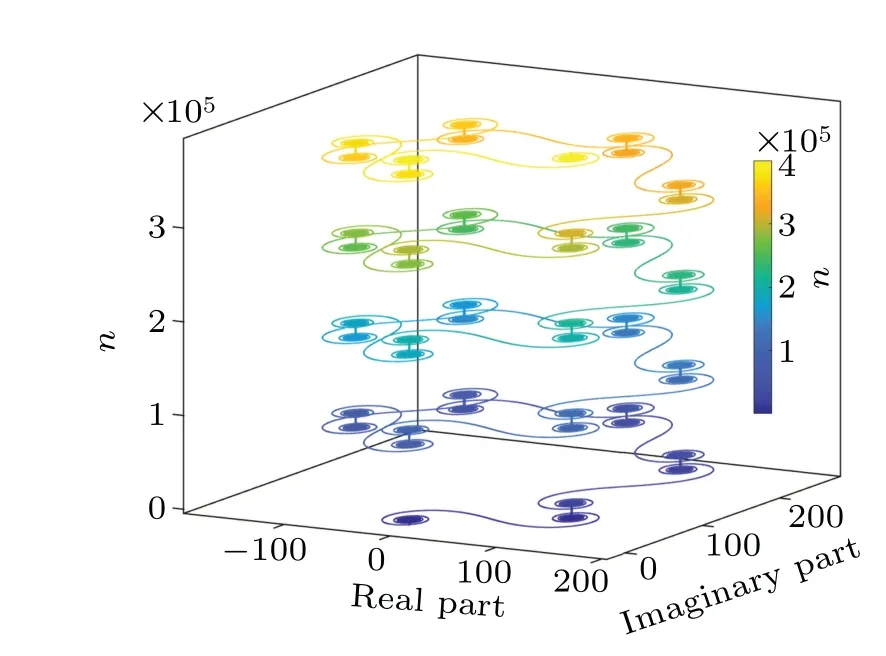
Fig. 5. The characteristic sum S(n) with α = 5/3, q = 1, and d =80000/3. The colors represent n,corresponding to the number of terms to be summed in the calculation of the characteristic sum S(n).

The rotational symmetry reads

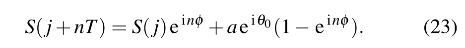
whereaeiθ0is the position of the center of symmetry. eiφis the rotational operator.φis the least invariant angle. The least invariant angle means the least angle to hold the rotation invariance in the complex number space. For example,the least invariant angle depicted in Fig.5 isπ/3.Tis the least rotation period.

The characteristic sumS(j+nT)reads

Ifnφis a multiple of 2π,thenS(j+nT)=S(j). The leastnφis the dynamical evolution period of the fractional resonance case. Through lettingn=1 in Eq.(23),we have the following equations:

After subtracting equations in Eq. (24) and substituting the characteristic sum expression forS(j) andS(j+1), respectively,

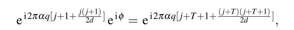
and canceling out the similar terms in the above equation,we get

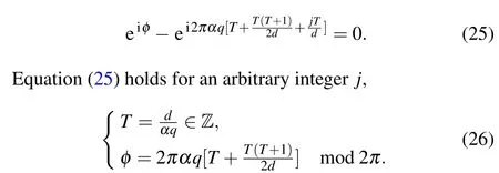
Equation(26)is the antiresonance condition of the characteristic sum with fractional values ofαqandd.

6. Experiment proposal

In this section,the experiment proposals for the LDQRM will be introduced. In Ref.[49],several experiment proposals have been devised to check the numerical results of the single QRKR and the coupled QRKR. The experimental proposals in this paper refer to their experiment proposals and modify them. Based on the Floquet operator expression in Eq. (2),one notices that the quantum dynamics are similar after exchanging the free Hamiltonian and the kicking potential in the Floquet operator.[49]In their experimental proposals,the original kicking potential is swapped for the free Hamiltonian. The swapping LDQRM Hamiltonian reads According to Eq. (3), the swapping exchanges the operating sequence of the free Hamiltonian part and the kicking potential part of the Floquet operator.

The experimental proposals proposed in this section include the realizations of the original LDQRMM and the swapping Hamiltonian of the LDQRMM in the novel optical lattice system, pulsed with the external magnetic field. In the first proposed experiment,the spin-1/2 particle hops in the 1D optical lattice,periodically pulsed by an external magnetic field.The 1D single-band tight-binding lattice provides the discrete lattice coordinates corresponding to the discrete dimensionless angular momentum eigenvalues in the LDQRMM. Table 1 summarizes the corresponding relationship between the LDQRMM and the spin-1/2 particle model mentioned here.

Table 1. Corresponding relationship.

In the table,ais the lattice constant. The quasimomentum in the first Brillouin zone is indexed ask. The quasi-momentum in the experiment corresponds to the angular coordinatexin the LDQRMM.The eigenvalue of the angular momentum operator ˆpin the LDQRMM corresponds to the index of the real space sitejin the 1D tight-binding lattice.µis the magnetic moment of the spin-1/2 particle.Bx(1)is thexcomponent of the magnetic field in the 1D lattice where the lattice index is 1.Bx(j)is thexcomponent of the magnetic field at the site of the 1D lattice indexed withj.Bx(j)=jBx(1).Tis the jumping energy that corresponds to the kicking strengthkin the LDQRMM. The Hamiltonian of the experiment system is

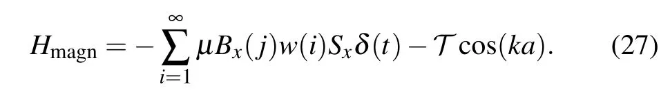
TheHmagnis the Hamiltonian of the first experiment system.irepresents the time of kicks.jrepresents the number of lattice sites. Unlike the experimental proposal designed for the original Maryland model,the experimental proposal in this paper adjusts the magnitude of the external magnetic field for the time of kicks.w(i) is set to increase linearly over timeithroughw(i)=1+(i−1)/d. The magnitude of the magnetic field is proportional tow(i).

As we have mentioned in this section,after the exchange of the free and kicking part of the Hamiltonian,the dynamical evolution pattern is similar.Hmagnis the swapping Hamiltonian of the LDQRMM. The Hamiltonian of another experimental proposal readsHpl,which describes a spin-1/2 particle that is in the constant magnetic field, pulsed with an optical lattice potential. The Hamiltonian reads

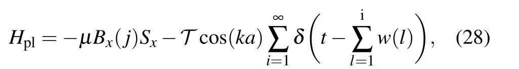
wherew(l) is the sum of the linearly delayed increases, andSxis the first component of the Pauli matrix operator. To prevent the free Hamiltonian return to the quadratic kinetic energy form,the kicking operation is simulated by switching the deep lattice to the shallow one back and forth instead of completely turning on and off.[49]

In summary, the LDQRMM experiment proposals include two operating experiment frameworks. The first framework performs a linearly increasing magnetic field on a spin-1/2 particle in the optical lattice. The second proposal holds a constant magnetic field and lets spin-1/2 particles linearly delayed pulsed by an optical lattice potential.

7. Conclusion

This paper has discussed the evolution characteristics of the spread of angular momentum in the LDQRMM and LDCMM, including the resonance and antiresonance phenomenon with different system parameters. Our conclusions are listed below. Compared to the other cases of QRKR dynamical localization,the massless case(the Maryland model)shows the periodic evolution of the spread of the angular momentum.[48]To answer whether periodic kicks cause a periodic change of the angular momentum in the Maryland model,we have considered the LDQRMM,a non-periodically kicked Maryland model, in this paper. We found that the resonance and antiresonance phenomenon of the angular momentum spread exist in the LDQRMM. In Sections 2–5, the resonance and antiresonance phenomenon in the LDQRMM are interpreted through classifications and discussions of the characteristic sum. In the LDQRMM,the antiresonance phenomenon appears with rational number parameters. It shows that the antiresonance phenomenon in the LDQRMM is more complex than that in the original Maryland model. The topology difference between different antiresonance cases emerges in the LDQRMM. It is also absent in a periodically kicked Maryland model.

Moreover, our work in this paper predicts some localization phenomena in the corresponding 1D tight-binding lattice. We argue that the LDQRMM can be realized by hopping spin-1/2 particles in a 1D tight-binding lattice. This 1D tightbinding lattice is pulsed with a linearly delayed magnetic field in thex-direction. The wave function spread of a spin-1/2 particle in the optical lattice corresponds to the evolution of the angular momentum spread in the LDQRMM.

Acknowledgements

Project supported by the Science and Technology Development Fund (FDCT) of Macau, China (Grant Nos.0014/2022/A1 and 0042/2018/A2)and the National Natural Science Foundation of China (Grant Nos. 11761161001,12035011,and 11975167).