WANG Shuwen, YANG Kunde, 3), SHI Yang, *, YANG Fan, and ZHANG Hao

Impact of Evaporation Duct on Electromagnetic Wave Propagation During a Typhoon

WANG Shuwen1), 2), YANG Kunde1), 2), 3), SHI Yang1), 2), *, YANG Fan1), 2), and ZHANG Hao1), 2)

1) School of Marine Science and Technology, Northwestern Polytechnical University, Xi’an 710072, China 2) Key Laboratory of Ocean Acoustics and Sensing, Northwestern Polytechnical University, Ministry of Industry and Information Technology, Xi’an 710072, China 3) National Key Laboratory of Underwater Information Processing and Control, Xi’an 710072, China

The evaporation duct, a result of evaporation from the ocean, is a region above the sea surface in which radio waves are refracted downward. This duct has strong effects on microwave instruments. Typhoons cause huge anomalies in marine meteorologi- cal parameters that influence the evaporation duct distribution and structure, which in turn affects the propagation of electromagnetic (EM) waves. However, EM wave propagation under the typhoon process has seldom been reported. Thus, taking Typhoon Phanfone (201929) as an example, this study uses a dataset from the European Centre for Medium-Range Weather Forecasts, combined with the Naval Atmospheric Vertical Surface Layer Model and the parabolic equation model, to study the evaporation duct’s impact on EM wave propagation during a typhoon. The spatial and temporal path loss distributions reveal that large amounts of EM wave en- ergy are emitted from the evaporation duct when the EM wave passes through a typhoon eye. On average, a typhoon eye causes an approximately 20 dB increase in path loss for EM wave propagation at low antenna height. Furthermore, the effects of a typhoon eye on EM wave propagation at different signal frequencies and antenna heights are studied. The results show that a typhoon has a larger impact on EM wave propagation with low signal frequency and high antenna height.

evaporation duct; typhoon; ECMWF; wave glider; electromagnetic wave propagation

1 Introduction

Evaporation ducts are formed at the air-sea boundary as a result of the gradual decrease in humidity from the sea surface upwards. In the evaporation duct layer, the elec- tromagnetic (EM) waves are refracted to the sea surface and behave like they are trapped in this layer (Babin, 1996; Babin and Dockery, 2002). The evaporation duct has con- siderable effects on maritime radar, communication, navi- gation and other microwave instruments, especially those operating above 3GHz (Shi, 2015a, 2015b). The evaporation duct height (EDH) defines the strength of the duct and can be determined by different methods, such as direct measurements (Liu, 1979), inversion methods (Yardim, 2007; Saeger, 2015; Wang, 2019), and numerical models (Paulus, 1985; Mussongenon, 1992; Frederickson, 2000, 2003; Frederickson, 2015; Zhang, 2017). The evaporation duct is almost always present over the global ocean, and several studies have presented global and regional evaporation duct climatol- ogy (Twigg, 2007; Frederickson, 2008; Ding, 2010; McKeon, 2013; Shi, 2015c; Sirkova, 2015; Zhang, 2016).

The parabolic equation (PE) has been widely used to model radio-wave propagation in the troposphere for over-ocean paths. The advantage of using the PE method is that it provides a full-wave solution for the field in the pres- enceofrange-dependentenvironments(Barrios,1994).Nu- merous models based on the PE method have been de- veloped, such as the Terrain Parabolic Equation Model (TPEM) (Barrios, 1994), the Parabolic Equation Toolbox (PETOOL) (Ozgun, 2020) and the Advanced Propa- gation Model (APM) (Barrios and Patterson, 2002). Sev- eral field experiments (Hitney and Vieth, 1990; Anderson, 2004; Woods, 2009; Wang, 2018) on EM wave propagation in the evaporation duct environment have also been conducted. Thus far, studies have shown that the EDH, the antenna, and the frequency in use are important factors in determining the propagation loss.

Although the evaporation duct model and the EM wave propagation model have become more accurate in recent years, researchers have maintained that there exists a cer- tain gap between the measured path loss and the simu- lated one (Woods, 2009; Shi, 2015a). This is because the marine environment and the atmospheric en- vironment are constantly changing dynamically. The EDH is greatly affected by marine meteorological parameters, such as wind speed, pressure, air temperature, sea surface temperature, and specific humidity. Thus, the evaporation duct varies widely with the weather and seasons, some- times changing from strong to non-existent in a single day. Recently, the development of numerical evaporation duct models and reanalysis data (Saha, 2014; Sirkova, 2015; Hersbach, 2020) has made it possible to ob- tain information on the large-area, long-term and hori- zontal inhomogeneous variability of the evaporation duct. The influence of the evaporation duct on the propagation of EM waves can be well investigated by considering the spatial and temporal inhomogeneity of the evaporation duct. In summary, studies so far have focused on the influ- ence of complex, inhomogeneous, and dynamically chang- ing maritime environments on EM wave propagation.

Typhoons are mature tropical cyclones that form over warm ocean waters in the Northwest Pacific, and their outer circulation can extend more than 1000km from the typhoon center. Typhoons cause extremely high sustained surface winds of 33ms−1or higher, torrential rains and storm surges (Montgomery and Farrell, 1993). Dozens of typhoons form year-round in the Northwest Pacific–knownas a hotbed of typhoons–and the most intensive period occurs from May to October every year (Cheung, 2013). During typhoons, the ocean meteorological para- meters, such as wind, pressure, and temperature, are greatly affected. Typhoons result in substantial air-ocean interac- tions that then affect the evaporation of the sea surface.

More recent studies have shown that ducts are likely to be formed on the periphery of a tropical cyclone (TC) and in its eye. For instance, in their analysis of an unusual radar abnormal propagation phenomenon associated with foehn winds induced by Typhoon Krosa (200715), Chang and Lin (2011) found that significant subsidence warming and drying from downslope winds provided favorably envi- ronmental conditions for the duct occurrences. Liu(2012) used the Weather Research and Forecasting (WRF) model to study the atmospheric duct process during Ty- phoon Rusa (200215). They found that humidity gradient is a key factor in the formation of this duct and that the temperature inversion enhances its strength. Ding(2013) analyzed the statistical characteristics of the ducts induced by TCs over the western North Pacific Ocean for the period of September 2003 to September 2006 using the global positioning system (GPS) dropsondes in or around typhoons deployed by the ‘Dropsonde Observation for Typhoon Surveillance near the Taiwan Region (DOTS-TAR)’ program. They found 212 cases that showed ducting conditions of the total 357 dropsondes. Based on these GPS data, Fei(2013) investigated the impacts of the bogus data assimilation and sea spray parameterization on the typhoon duct using the WRF model. Notably, they found the simulated surface ducts to the south and east of the typhoon center are actually evaporation ducts. How- ever, due to the still poor vertical resolution of the model in the surface layer, their results needed further verifica- tion.

Owing to the development of numerical evaporation ductmodels and high-resolution reanalysis data, it has now be- come possible to study the distribution of evaporation ductsduring typhoons. For example, Shi(2019) studied the influence of typhoons on the evaporation duct distribution using the Naval Atmospheric Vertical Surface Layer Model (NAVSLaM) and found that the trajectory of the typhoon center is almost the same as that of the EDH minimum center. Previous studies have also shown that typhoons are indeed conducive to the formation of atmospheric ducts and can cause abnormal propagation of EM systems, such as radars(Chang and Lin, 2011). However, these studies have mainly focused on high-altitude ducts and rarely studied their effects on EM propagation. Thus, the purpose of the current study is to investigate the influence on EM wave propagation of the special evaporation duct structure during typhoons.

The rest of the paper is organized into sections. Section 2 presents the materials and methods that are used to study the distribution of the evaporation duct during typhoons, along with the propagation of EM waves in the evapora- tion duct are presented. Section 3 discusses the reanalysis data validation using data from buoys and wave gliders. Section 4 presents a comparison of EM wave propagation in the evaporation duct with and without a typhoon eye. Section 5 discusses the influence of the typhoon eye on EM wave propagation at different signal frequencies and antenna heights. Finally, Section 6 provides the conclu- sion.

2 Materials and Methods

This study used the European Centre for Medium-Range Weather Forecasts (ECMWF) ERA5 dataset and the NA- VSLaM to calculate the EDH distribution during the ty- phoon, which we then combined with the APM to study the impacts of the evaporation duct on EM wave propa- gation during the typhoon process. A research flow dia- gram of this study is shown in Fig.1. First, the required atmospheric parameters, such as air temperature, atmos- pheric pressure, specific humidity, sea surface tempera- ture, and wind speed, were extracted from the ECMWF ERA5 dataset. Second, the meteorological data monitored by buoys and wave gliders during the typhoons were used to verify the reliability of the ECMWF data. Third, the above parameters were brought into the NAVSLaM to calculate the EDH distribution during the typhoon. Fourth, the obtained EDH distribution was used as the input of the PE model. Finally, the effects of the evaporation duct structure with a typhoon eye on the propagation of EM waves were analyzed by combining different EM wave frequencies, antenna heights, and receiving distances.

2.1 Evaporation Duct Model

At present, the evaporation duct prediction model is the main method for obtaining the height of the evaporation duct and its vertical distribution of the modified refractive index. The EDH is a crucial parameter for measuring the evaporation duct and can be used to describe the ability of the evaporation duct layer to trap EM waves. In such a layer, the atmospheric modified refractivity profilede- creases as the sea surface height increases. When a certain height is reached, the modified refractivity reaches a mini- mum value and then increases with height. The height cor- responding to the minimum point is defined as the EDH.The modified refractivitycan be expressed as a com- bination of air temperature(K), total atmospheric pres- sure(hPa), partial pressure of water vapor(hPa), and the height above sea surface(m) as follows:

In recent years, several evaporation duct models, such as the Paulus-Jeske (PJ) model (Paulus, 1985), the Mus- son-Gauthier-Bruth (MGB) model (Mussongenon, 1992), the Liu-Katsaros-Businger (LKB) model (Babin and Dockery, 2002), the Babin-Young-Carton (BYC) model (Babin, 1996), and the NAVSLaM (Frederickson, 2015), have been developed to calculate the-profiles and EDHs. The NAVSLaM is an evaporation duct prediction model developed by the US Naval Postgraduate Institute. It uses a total ocean-air flux algorithm obtained from long-term marine surveys (Liu, 1979) and is currently an offi- cial operational model for the US Navy. The NAVSLaM, which is based on the Monin-Obukhov Similarity (MOS) and LKB theories, uses the air temperature, atmospheric pressure, wind speed, and relative humidity at known alti- tudes as well as the average sea surface temperature to calculate the-profiles.

As shown in Eq. (1) below, the temperature, pressure, and partial pressure of water vapor profiles are needed to calculate the-profiles. The NAVSLaM derives these pro- files from the following equations:

where() and() present the air temperature and spe- cific humidity, respectively, at a given heightabove the sea surface;0and0qare the integration constants called the temperature and specific humidity roughness length, respectively; and*and*are the Monin-Obukhov tem- perature and specific humidity scaling parameters, re- spectively. The values of0,0q,*, and*are calculated using the TOGA COARE 3.0 bulk flux algorithm (Fairall, 2003). In addition,is von Karman’s constant; Γis the adiabatic lapse rate, which approximately equals 0.00976Km−1;is the Obukhov length;,, andcor- respond to gravity acceleration, gas constant for dry air, and constant value of 0.622, respectively;Tis the mean value of virtual temperature at heights of1and2;ψdenotes the temperature function and is given different for- mulas depending on whether the atmospheric layer condi- tions are unstable or stable/neutral; and/is defined as the Monin-Obukhov parameter that is used to express the stability of the atmosphere. Stable, neutral, and unsta- ble conditions are defined as>0,=0, and<0, respec- tively.

The NAVSLaM has been widely compared and verified by many profiling observations and through various EM wave propagation experiments under different meteoro- logical conditions. Babin and Dockery (2002) conducted a careful theoretical analysis and buoy data validation evaluation of the existing model and concluded that the NAVSLaM is an ideal model for estimating the EDH and the refractive index profile.The rough evaporation duct experiment (Anderson, 2004) was conducted off the shores of the Hawaiian Island of Oahu, and the experi- ment showed that the MOST can be used to accurately predict EM propagation by modeling the refractivity in the marine-atmospheric boundary layer. A fixed X-band array EM propagation experiment (Pozderac, 2018) was deployed at the 2013 SoCal experiment and Scripps Pier Campaign, and the results showed a strong correla- tion between the EM-inverted EDH and NAVSLaM-cal- culated EDH. A coupled air-sea processes and electromag- netic ducting research (Wang, 2018, 2019) conducted off the coast of Duck, NC, USA, during October–Novem- ber of 2015 also found a very good agreement between measurements and inversion results with the NAVSLaM modeling results.

The processed ECMWF ERA5 data were brought into the NAVSLaM, after which the distribution of the evapo- ration duct in the corresponding sea area during Typhoon Phanfone was obtained.

2.2 PE Method

The PE is the mainstream method for calculating EM wave propagation in the troposphere (Barrios, 1994). It can be used to calculate the propagation of EM waves in a range-dependent troposphere. The standard PE can be de- rived from the Helmholtz equation (Kraut, 2004) pre- sented as follows:

In Eq. (6) above,is the range,is the altitude,is the wave number,is the modified refraction index, andis a scalar component given by

whereis the electric or the magnetic field.

Eq. (6) can be solved by using the split-step Fourier technique as follows:

whereand−1are the Fourier transform and the Fourier inverse transform, respectively;=sin(), whererepre- sents the angle of propagation; andis the range incre- ment.

The APM model based on the PE method is typically used to investigate the effects of the special EDH struc- ture during a typhoon on EM wave propagation. The APMis a hybrid model that combines the radio physical optics (RPO) model and the terrain parabolic equation model (TPEM) in a relatively fast code. The APM is used in the advanced refractivity effects prediction system (AREPS), which is widely applied in the assessment of EM instru-ments. The APM has been validated and used in various evaporation duct environments along the propagation path (Barrios and Patterson, 2002; Shi, 2015a, 2015b).

3 Data

3.1 Typhoon Data

The typhoon data were obtained from the Japan Mete- orological Agency (Japan Meteorological Agency, 2019). Fig.2(a) shows the typhoon tracks in the Northwest Pacific Ocean in 2019. Typhoon Phanfone (201929) (as shown by the red line in Fig.2(a)), which passes through the Philip- pine Islands, is taken as an example to study the perform- ance of shore-based microwave instruments, such as radars, communication systems, and navigation systems, when a typhoon arrives. Fig.2(b) shows a meteorological satellite observation image of the typhoon (Kitamoto Laboratory JPN, 2019). Typhoon Phanfone (201929) (Wikipedia contributors, 2020) first formed as an upper-level low near the Caroline Islands on December 19, 2019 (UTC) and intensified into a tropical storm on December 22, moving generally in a west–north direction. Phanfone made its first landfall in Samar, Philippines, on December 24. Despite making several landfalls over the central Philippine islands, its intensity continued to increase until December 25. After exiting the Philippine landmass, Phanfone maintained its typhoon strength for several hours and finally dissipated over the South China Sea on December 28. Phanfone’s basic information is shown in Table 1.

Table 1 Basic information on Typhoon Phanfone

Fig.2 (a) The typhoon tracks in the Northwest Pacific Ocean in 2019 (red line: Typhoon Phanfone). (b) Meteorological satellite observation image of Typhoon Phanfone (201929).

3.2 Reanalysis Data

The reanalysis products can provide the long-term, global,high-spatial-resolution and high-temporal-resolution atmos- pheric data near the sea surface, which can then be used to calculate the large-area, long-term, and horizontal in- homogeneous evaporation duct distribution. The ECMWF ERA5 hourly data were used in the current study to cal- culate the distribution of the evaporation duct. ERA5 (Hersbach, 2020) is the fifth-generation ECMWF atmospheric reanalysis of the global climate with tempo- ral coverage from 1979 to the present. ERA5 combines model data with observations from across the world into a globally complete and consistent dataset using the laws of physics, which is called data assimilation. The time reso- lution of ERA5 is 1h, and the spatial resolution is 0.25˚×0.25˚. Due to the global coverage and high resolution, this dataset is suitable for use in analyzing the evaporation duct structure during typhoons.

As Typhoon Phanfone took place in December 2019, the ERA5 data for December 2019 were extracted. The extracted parameters included the air temperature at 2m, atmospheric surface pressure, wind speed at 10m, spe- cific humidity at 2m, and the sea surface temperature.

3.3 Validation of Reanalysis Data

Independent observations are needed for comparison in order to verify the reliability of the ECWMF data during typhoons. In this section, we used the observation data of both the mooring equipment and mobile observation equip- ment to verify the reliability of the reanalysis data during typhoons. First, the buoy observation data were used to verify the ECMWF data during typhoons. Moreover, a wave glider was deployed in the western Pacific to observe the marine environment during the typhoon. The observa- tion data were also used for the reanalysis data validation.

3.3.1 Verification by buoy data

To verify the ECWMF data under different typhoonstructures, we used the buoy data that were measured when the typhoon eye passed the buoy. Buoy data are consid- ered the best benchmark data because the buoys are often located in the open sea and are less affected by the main- land and research platforms (Newton, 2003). The Triangle Trans-Ocean buoy Network (TRITON) buoy (Kuroda and Amitani, 2001) was used to verify the ECWMF data dur- ing the typhoon. The TRITON is a series of buoys deploy- ed by the Japan Agency for Marine-Earth Science and Tech- nology (JAMSTEC) for measuring surface meteorology and the upper ocean. Fig.3 shows the TRITON buoy and its meteorological sensors.

Around December 22, 2019, Typhoon Phanfone passed the TRITON buoy moored at 8˚N, 137˚E. Fig.4 shows the track of Typhoon Phanfone and the TRITON buoy loca- tion. The daily buoy observation values of air temperature (AT), sea surface temperature (SST), air pressure (AP), wind speed (WS), and relative humidity (RH) from De- cember 19–31, 2019, were used for comparison. The data from the ECMWF reanalysis grid point nearest to the buoy location were extracted, and the daily means of those data were obtained by averaging the hourly values. Subse- quently, the EDHs were obtained by bringing the above meteorological data and their measured heights into the NAVSLaM. A comparison of the ECMWF data with buoy observation data is shown in Fig.5. Meanwhile, Table 2 shows the average differences of meteorological data and EDHs between the ECMWF data and the buoy data dur- ing Typhoon Phanfone.

Table 2 Average differences between reanalysis data and buoy data

In general, as shown in Fig.5, ECMWF data agreed well with the buoy data. The differences between the reanaly- sis data and the buoy data could be attributed to the data assimilation techniques or the insufficient observations. In addition, the datasets both captured the changes in me- teorological parameters during the passing of Typhoon Phanfone’s eye (around December 22, 2019), which com- prised sharp drops in WS and AP.

As revealed in Fig.5(f), the ECMWF-based EDHs show- ed good agreement with buoy-based EDHs, with an av- erage difference of about 1.3m. The EDH difference be- tween the ECMWF data and the buoy data was larger on December 22, 2019, which was 3.1m. This may be attrib- uted to the notable WS error when the typhoon came. In addition, the calculated EDHs also showed an interesting drop on December 22, just like the WS and AP. Then, as the typhoon center moved away, the EDH increased due to the higher WS at the periphery of the typhoon. There- fore, it can be preliminarily inferred that the arrival of a typhoon affects the distribution of the evaporation duct.

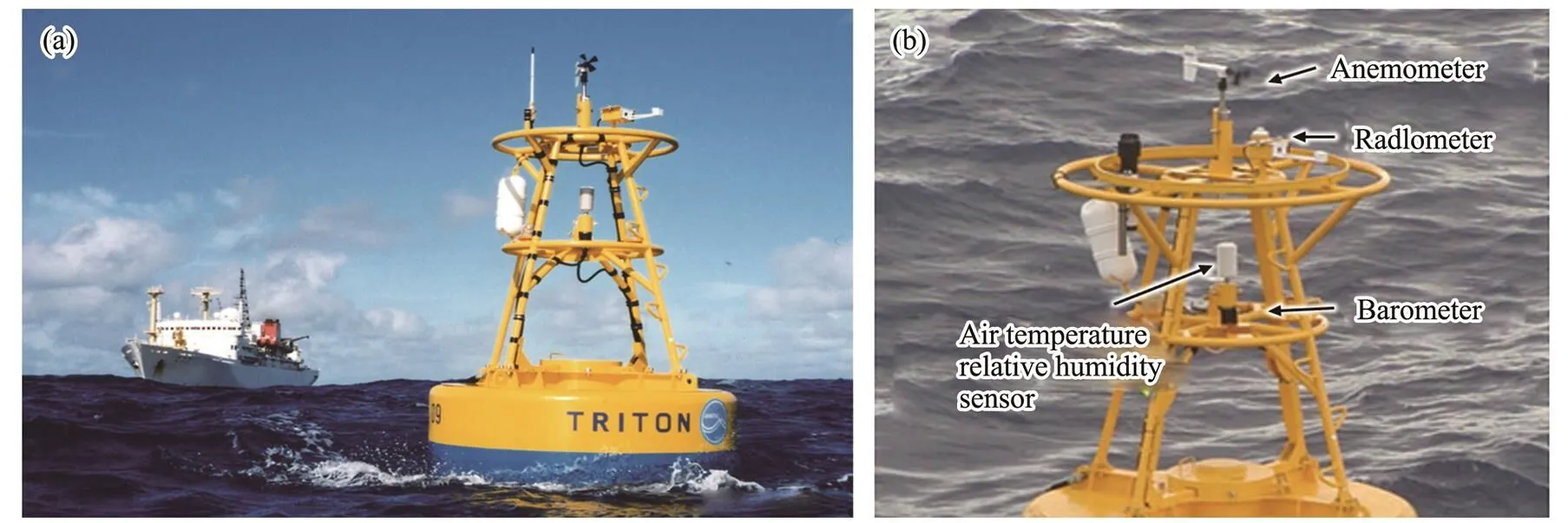
Fig.3 (a) The TRITON buoy. (b) The meteorological sensors.

Fig.4 The track of Typhoon Phanfone, showing the intensity and arrival time of the typhoon and the location of the TRITON buoy. Line, typhoon track; pentagram, TRITON buoy location; large points, the position of the typhoon each day at 00:00 UTC (the number in the circle represents the ‘day’); small points, the position of the typhoon every 3–6h; blue points, tropical depression (class 2); green points, tropical storm (class 3), yellow points, severe tropical storm (class 4); red points, typhoon (class 5).

Fig.5 Comparison of meteorological parameters and calculated EDHs between the ECMWF data and the buoy observation data during Typhoon Phanfone (2019 UTC). (a)–(e), Meteorological parameters; (f), EDHs.

Overall, the results show that the ECMWF data can be used to reliably model and assimilate the marine envi- ronment. These comparisons suggest that applying the ECMWF dataset to calculate the EDH during a typhoon is a reliable approach.

3.3.2 Verification by wave glider data

Buoys are usually anchored, and only a fixed point of the marine environment during the typhoon can be observed. Therefore, to thoroughly verify the reliability of the re- analysis data, a wave glider, which can sail around, was used to observe a wide range of the marine environment when a typhoon arrived. An observation experiment was held on September 7–27, 2019 (UTC), using a wave glider called Black Pearl (Li, 2017; Sun, 2019) (Ocean University of China, Qingdao, Shandong, China; Tsingtao Hydrotech Co., Ltd., Qingdao, Shandong, China). The pur- pose was to observe changes in the marine environment during a typhoon. The tracks of the wave glider and the observed Typhoon Faxai (201915) are shown in Fig.6. The wave glider was equipped with an automatic weather sta- tion and water temperature sensor. The configurations of the sensors are shown in Table 3. The wave glider recorded a set of AT, SST, RH, AP, and WS data approximately every 10min. In addition, the longitude, latitude, speed, sailing direction, pitch angle, voltage and other informa- tion of the wave glider itself were also recorded.

The data from the ECMWF reanalysis grid point near- est to the wave glider location were extracted at the hour points that were closest to the data recording time of the wave glider. A comparison of the meteorological parame- ters between the ECMWF data and the wave glider ob- servation data during Typhoon Faxai is shown in Fig.7(a)–(f). First of all, it is important to note that the RH meas- ured by the glider was invalid because the weather station was installed close to the sea surface, which was only about 2m high. This caused the sensor to become wet and invalid, which in turn led to inaccurate humidity meas- urements. Therefore, the humidity measured by the wave glider was replaced by the humidity in the reanalysis data when calculating the EDH using the wave glider data. It can be seen from Fig.7 that the SST, AP, and WS of the reanalysis dataset showed good agreement with the wave glider measurement data. Furthermore, the difference in AT between the ECMWF data and the wave glider data was 2.8℃ on average. Overall, the reanalysis datasets showed good agreement with the wave glider data, with some small gaps. Apart from the errors caused by the reanalysis proc- ess, these small gaps may also be due to the fact that the compared data were not at the exact same spatial locations and time points. The wave glider observed the meteoro- logical data of a single point per 10 seconds, and the posi- tions of the data point changed with time. However, the extracted reanalysis data were hourly average data with a spatial resolution of 0.25˚×0.25˚. Moreover, the average distance between the two datasets points was about 10km, and the maximum can reach 17km.

Fig.6 (a) The track of Typhoon Faxai and the wave glider. Line, Typhoon Faxai track; cyan points, wave glider locations; magenta points, extratropical cyclone (class 6). Refer to Fig.4 for other notes. (b) The wave glider.

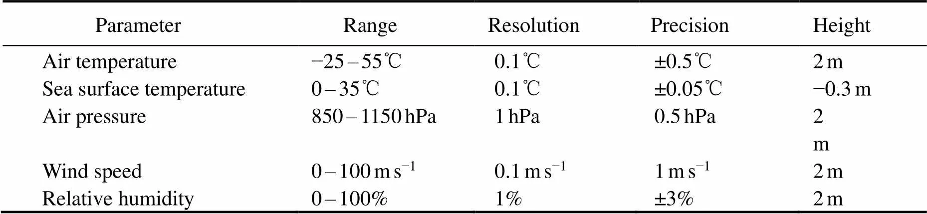
Table 3 Configurations of the sensors

Fig.7 Comparison of meteorological parameters and calculated EDHs between the ECMWF data and the wave glider observation data during Typhoon Faxai (2019 UTC).

The calculated EDHs and their absolute differences are shown in Figs.7(g) and (h), respectively. The EDHs cal- culated by ECMWF showed good agreement with the glider’s value most of the time. However, there were also large differences (around 10m) at some moments due to differences in meteorological factors. The main reason for the large differences can be attributed to the values of AS- TD. As shown in Fig.7(h), the green dots indicate the mo- ments when the sign of the ASTD for ECMWF and the wave glider are the opposite. In these moments, the atmos- pheric layer conditions between the two datasets varied,which then led to differentψfunctions in the NAVSLaM model and eventually resulted in huge EDH differences between ECMWF and the wave glider.

Although there were some gaps between the ECMWF data and wave glider measured data, overall, the difference in EDH deviation fell within an acceptable range. Com- parisons with wave glider observation data also confirm that the ECMWF data are suitable for studying the distri- bution of EDHs during a typhoon.

4 Results

A comparison of the EM propagation with and without a typhoon eye is presented in this section. Then, the spa- tial and temporal distributions of path loss with and with- out a typhoon eye are presented. This is followed by a discussion of the effects of the typhoon eye on EM wave propagation at different signal frequencies and antenna heights. Furthermore, the EM propagations inside the evap- oration duct during other typhoons are also analyzed to verify the universality of the conclusions.

The hourly distribution of the evaporation duct during Typhoon Phanfone was calculated using the ECMWF ERA5 data and the NAVSLaM. Typhoon Phanfone had an important effect on the EDH distribution: there was an ‘evap- oration duct eye’ with a very low EDH in the typhoon eye. Fig.8 shows the trajectory comparison of the Typhoon Phanfone center and the EDH minimum center, in which the blue line represents the typhoon center and the red cir- cles representing the EDH minimum center. As can be seen, these two tracks are nearly coincident.

Fig.8 Track of the Typhoon Phanfone center and the EDH minimum center. Blue line, Typhoon Phanfone center; Red circles, EDH minimum center.

Fig.9 shows the distributions of the EDH, WS, AP, RH, SST, and AT 19:00 on December 25, 2019 (UTC). The center of Phanfone at this time was located near 12.8˚N, 119.4˚E. Typhoon Phanfone was moving toward the west-northwest direction and had maximum sustained winds approaching 65kt. In addition, there was a distinct EDH minimum center at 12.75˚N, 119.5˚E (P2). These two cen- ters were quite close. During the typhoon, WS and AP showed a distinct minimum center, similar to the distribution of the EDH. RH had a less obvious minimum central distribution, but the temperatures did not show this dis- tribution.

We chose 19:00 on August 25, 2019 (UTC) as an ex- ample with a typhoon eye in order to study the effect of the evaporation duct structure with a typhoon eye on EM wave propagation. We intersected the EDH structure, rang- ing from 118.25˚E to 120.75˚E, along 12.75˚N, as shown by the blue circles in Fig.9(f). In addition, the time point of 21:00 on August 19, 2019 (UTC) was also selected as a comparison representing the evaporation duct structure without a typhoon eye.

Fig.10 shows the AT, SST, AP, WS, RH, and EDH along this intersect at these time points. With a typhoon eye, the EDH was 15m at 118.25˚E, fell to a minimum (about 7.5m) at 119.5˚E (the typhoon eye), and then began to in- crease again. The EDH without a typhoon eye remained around 15m. WS and AP showed similar trends. In short, when the typhoon eye is present, the evaporation duct struc- ture is concave.

Fig.9 Atmospheric factors (a–e) and EDH (f) distributions at 19:00 on December 25, 2019 (UTC).

As shown in Fig.9(f), the transmitting antenna was lo- cated on the western side of Mindoro Island, Philippines, at 12.75˚N, 120.87˚E (P1). The propagation path was up to 285km and ended at 12.75˚N, 118.25˚E (P3). Mean- while, Fig.11 shows the modified refractivity profiles of the cases with and without a typhoon eye along the propa- gation path. These profiles were inputted into the APM to calculate the path loss. The EM wave frequency was 8GHz, and the transmitting antenna height was assumed to be 5m.

4.1 Comparison of the EM Propagation with and Without a Typhoon Eye

Fig.12 shows a comparison of the path losses with and without the Phanfone typhoon eye. By comparing Figs.12(a) and (b), we can clearly see that the EM waves were trapped in the evaporation duct layer; however, as the EM waves passed through the typhoon eye, a large amount of EM wave energy was emitted from the evaporation duct. This can also be verified from Fig.12(c), which indicated that the path loss varied with the propagation distance at the receiving antenna height (RAH) of 5m. There was a sharp increase (about 58dB increase from 130–170km) in path loss when the EM waves passed through the ty- phoon eye. The path loss at the receiving distance (RD) of 285km was approximately173.7dB with a typhoon eye, while the path loss was about 145.2dB without one. The typhoon eye caused an approximately 28.5dB increase in the path loss.

Meanwhile, Fig.12(d) shows the variation of path loss with height at RD 148km (typhoon eye). The path losses at a receiving height of 5m with and without a typhoon eye were 150.1 and 141.7dB, respectively. However, at a receiving height of 60m, the path losses with and without a typhoon eye were 153.5 and 193.1dB, respectively. The path loss with a typhoon eye was larger when the receiv- ing height was low but smaller when the height was high. This was because the EM wave leaked out of the evapo- ration duct layer and reached a higher position. This in- teresting phenomenon may enable a land-based radar to detect an aircraft above the eye of a typhoon beyond the visual range. Fig.12(e) shows the variation of path loss with height at an RD of 285km. The path losses at a re- ceiving height of 5m with and without a typhoon eye were was 145.2 and 173.7dB, respectively. In both cases, EM waves were still trapped by the evaporation duct layer, and the path loss was minimal at an antenna height of around 5m. However, owing to the energy leakage, the typhoon eye caused an approximately 20dB increase in path loss, on average, at an RD of 285km.

Fig.10 EDH and atmospheric factors structures.

Fig.11 The modified refractivity profiles along the propagation path. (a), With a typhoon eye; (b), Without a typhoon eye.

4.2 Spatial Distributions of Path Loss with and Without a Typhoon

Fig.13 shows the spatial distributions of path losses with and without a typhoon eye. As can be seen, the transmit- ting antenna was still located at 12.75˚N, 120.87˚E (P1). The signal frequency was 8GHz, and the transmitting an- tenna height was 5m. The distributions of the evaporation duct of a sector with a radius of 300km were extracted, after which the path loss distributions at RAHs of 5 and 60m were obtained. As shown in Fig.13, when the EM wave passed through the typhoon eye, the path loss at an RAH of 5m increased, while the path loss remained small in other directions. However, the path loss decreased at an RAH of 60m when the EM wave passed through the ty- phoon eye. This can be attributed to the low EDH at the typhoon eye, which caused the EM wave energy to leak to a high position.

4.3 Temporal Variations of Path Loss During a Typhoon

Fig.14 shows the temporal variation of path loss during December 25, 2019, for Typhoon Phanfone. The system parameters are shown in Table 4 (Cases 1–4). For Case 1 (black line), where the RAH was 5m and the RD was 148km, the path loss was around 134dB before the arrival of the typhoon eye. Then, the typhoon eye passed the trans- mission path at around 18:00, and the path loss increased to about 153dB. Finally, the typhoon eye diverged from thetransmission path, and the path loss was restored to 140dB. However, when the RAH was 60m and the RD was still 148km (Case 2, blue line), the path loss decreased as Ty- phoon Phanfone passed by due to the EM energy leakage caused by the typhoon eye. For Case 3 (red line) and Case 4 (green line), where the RD was 285km, the path loss increased at both RAHs as the typhoon passed by. This was also due to the EDH being lower at the typhoon eye and the EM wave leaking out of the propagation path. There- fore, the typhoon process had a substantial impact on EM wave propagation. The main manifestation can be seen in the EM wave energy at the typhoon eye leaking upwards, resulting in a smaller path loss at a higher position at the typhoon eye and a larger path loss on the propagation path behind the typhoon eye.

Fig.12 Path loss distribution of EM wave propagation (P1–P3). (a), Path loss distributions with a typhoon eye and (b) without a typhoon eye; (c), Path loss at a receiving height of 5m; (d), Path losses at receiving distances of 148km and (e) 285km.

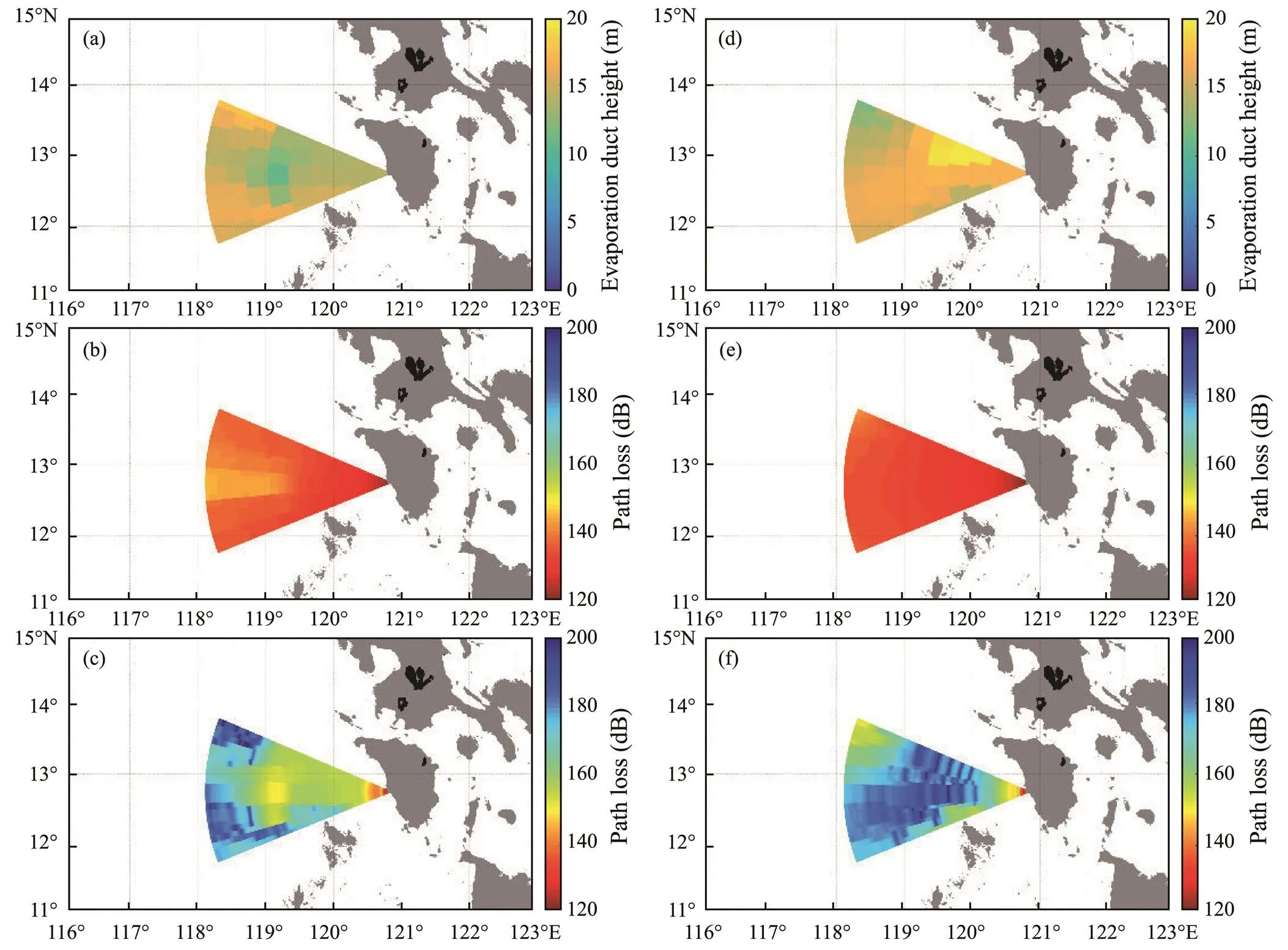
Fig.13 EDHs and path loss spatial distribution. (a), EDH spatial distribution with a typhoon eye; (b), Path loss spatial distributions with typhoon eyes at RAHs of 5m and (c) 60m. (d), EDH spatial distribution without a typhoon eye; (e), Path loss spatial distributions without a typhoon eye at RAHs of 5m and (f) 60m.

Fig.14 Path loss variation with time at frequency 8GHz.

Table 4 System parameters

4.4 Results for Other Typhoons

We also analyzed the EM propagation inside the evapo- ration duct during other typhoons to verify the universal- ity of the conclusions. The results were similar. In particu- lar, we present the results on Typhoon Lekima (201909), and the results are shown in Fig.15. The comparison be- tween the typhoon trajectory and EDH minimum center, shown in Fig.15(a), revealed great consistency. The EDH structure, ranging from 127.5˚E to 130˚E, was intersected along 19.25˚N on August 6, 2019, at 13:00 (UTC) to cal- culate the path loss distribution, shown by the blue circles in Fig.15(b). Figs.15(c)–(f) show a comparison of the path losses with and without the Lekima typhoon eye. As can be clearly seen, when passing through the typhoon eye, a large amount of EM wave energy was emitted from the evaporation duct. The typhoon caused an approximately 31.4dB increase in path loss at an RD of 263km and an RAH of 5m. The analysis results for Typhoon Lekima are consistent with those obtained for Typhoon Phanfone.

5 Discussion

Both the EM wave frequency and antenna height have a great influence on the EM wave propagation in the evap- oration duct. Therefore, this section discusses the effects of the typhoon eye on EM wave propagation at different signal frequencies and antenna heights.

Fig.16 shows the effects of the typhoon eye on EM wave propagation at different signal frequencies. The system parameters are shown in Table 4 (Case 5). Fig.16(a) showsthe path loss at signal frequencies ranging from 1–20GHz, which is the frequency band of concern for evaporation duct transmission. Fig.16(b) shows the difference between the path losses with and without a typhoon eye. When the EM wave frequency ranged from 1–3GHz, the path loss with a typhoon eye was almost the same as that without the typhoon eye. This can be attributed to the evaporation duct’s inability to trap EM waves at these frequencies and the fact that the changes in the evaporation duct caused by the typhoon had almost no effect on the propagation of the EM waves. As the frequency increased, the difference also increased with a maximum value of up to 58dB at 5GHz. Then, as the frequency increased, the ability of the evaporation duct to trap EM waves also increased, and therefore the difference diminished, reaching a minimum value of 1.2dB at 16GHz; after 16GHz, the gap increased slightly. The impact of the evaporation duct structure with a typhoon eye on the EM wave propagation becomes con- siderable when the frequency reaches around 4–12GHz.

The influence of the typhoon eye on EM wave propa- gation at different antenna heights is shown in Fig.17. The system parameters are shown in Table 4 (Case 6). In particular, Fig.17(a) shows the variation of path loss with antenna height ranging from 2–25m. When there was a typhoon eye, the path loss was larger at different antenna heights. Fig.17(b) shows the difference between the path loss without and with a typhoon eye. As can be seen, the difference in path loss between these two cases increased slowly as the height of the antenna increased to around 31dB at an antenna height of 15m, before remaining at around 31dB. This means that the influence of the evapo- ration duct structure with the typhoon eye on the EM wave propagation is smaller when the antenna height is lower. In addition, when the antenna is high, only the EM energy reflected from the sea surface continues to propa- gate in the evaporation duct layer due to the limitation of the height of the evaporation duct layer. The EM wave cannot propagate well in the evaporation duct layer; thus, the difference remains at around 31dB as the antenna height increases.

Fig.15 (a), Track of Typhoon Lekima center and the EDH minimum center. Blue line, Typhoon Lekima center; red circles, EDH minimum center; (b), Evaporation duct distribution (August 6, 2019 at 13:00 (UTC)); (c), Path loss distribution with a typhoon eye; (d), Path loss distribution without a typhoon eye; (e), Path loss at a receiving height of 5m; (f) Path loss at a receiving distance of 263km.

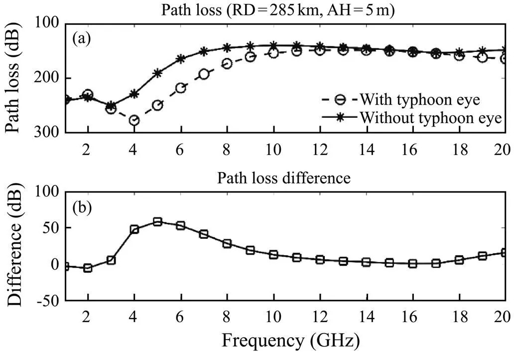
Fig.16 Influence of typhoon on EM wave propagation at dif- ferent signal frequencies. (a), Path loss variation with frequen- cy at an RAH of 5m and an RD of 285km; (b), Path loss dif- ference.

6 Conclusions

The influence of the evaporation duct structure on EM wave propagation during a typhoon was investigated in this study. The ECWMF data proved to be reliable in cal- culating the EDH during a typhoon compared to buoy ob- servation data and wave glider observation data. Further- more, the evaporation duct during a typhoon had a signifi- cant effect on EM wave propagation near the sea surface. The following conclusions are obtained in this paper:

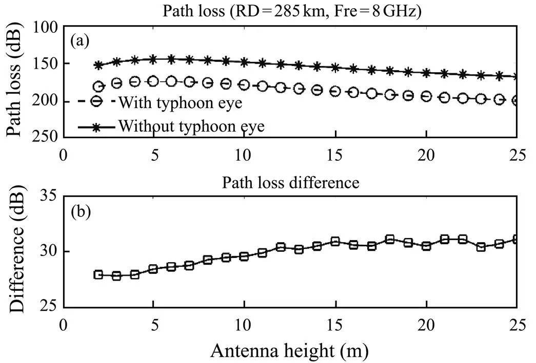
Fig.17 Influence of typhoon on EM wave propagation at dif- ferent antenna heights. (a), Path loss variation with antenna height at an RD of 285km and a frequency of 8GHz; (b), Path loss difference.

1) There was a distinct EDH minimum center during Ty- phoon Phanfone.

2) A comparison of the EM wave propagation in the spe- cial evaporation duct structure with and without a typhoon eye was presented. When propagating to the typhoon eye, a large amount of EM waves leaked out of the evapora- tion duct layer. Furthermore, the typhoon eye caused a 58dB increase from 130 to 170km in path loss for EM wave propagation. Compared to the moment without a typhoon eye, the path loss at the typhoon eye was 8.4dB larger at the receiving height of 5m but 40dB smaller at the re- ceiving height of 60m. This interesting phenomenon may result in a land-based radar being able to detect an aircraft above the eye of a typhoon beyond the visual range.

3) The typhoon eye had a considerable impact on EM wave propagation at a frequency range of 4–12GHz, there- by causing a maximum increase in path loss of 58dB. Fur- thermore, the impact of a typhoon eye on path loss in- creased by 11% as the height of the antenna increased from 2 to 15m.

This study, however, only studied the influence of the evaporation duct structure itself on EM wave propagation during a typhoon. In the future, experimental verification is needed, and the path loss data observed during the ty- phoon should be used to verify the conclusions of this work.

Acknowledgements

This work was supported in part by the National Natural Science Foundation of China (Nos. 42076198 and 41906160), and in part by the Innovation Foundation for Doctor Dissertation of Northwestern Polytechnical University (No. CX2022008). The authors would like to thank Professor Xiujun Sun and his team from the Ocean University of China for providing the wave glider observation data used in this paper. The authors also would like to thank Japan Meteorological Agency, ECMWF and JAMSTEC for providing the typhoon track data, reanalysis data, and buoy data used in this paper. The typhoon track data, reanalysis data, and buoy data could be available through Japan Meteorological Agency 2019, Hersbach(2020) and Kuroda and Amitani (2001) respectively.

Anderson, K., Brooks, B., Caffrey, P., Clarke, A., Cohen, L., Crahan, K.,, 2004. The RED experiment: An assessment of boundary layer effects in a trade winds regime on micro- wave and infrared propagation over the sea., 85 (9): 1355-1366, https://doi.org/10.1175/BAMS-85-9-1355.

Babin, S. M., 1996. A new model of the oceanic evaporation duct and its comparison with current models. PhD thesis. Univer- sity of Maryland at College Park.

Babin, S. M., and Dockery, G. D., 2002. LKB-based evapora- tion duct model comparison with buoy data., 41 (4): 434-446, https://doi.org/10.1175/1520-0450(2002)041<0434:Lbedmc>2.0.Co;2.

Barrios, A. E., 1994. A terrain parabolic equation model for pro- pagation in the troposphere., 42 (1): 90-98, https://doi.org/10.1109/8.272306.

Barrios, A., and Patterson, W. L., 2002. Advanced propagation Model (APM) Ver. 1.3.1 computer software configuration item(CSCI) documents. Technical Document 3145. Space and Na- val Warfare Systems Center, San Diego, 339pp.

Chang, P. L., and Lin, P. F., 2011. Radar anomalous propaga- tion associated with foehn winds induced by typhoon Krosa (2007)., 50: 1527-1542, https://doi.org/10.1175/2011JAMC2619.1.

Cheung, H.-F., Pan, J., Gu, Y., and Wang, Z., 2013. Remote- sensing observation of ocean responses to typhoon Lupit in the Northwest Pacific., 34 (4): 1478-1491, https://doi.org/10.1080/01431161.2012.721940.

Ding, J. L., Fei, J. F., Huang, X. G., Cheng, X. P., and Hu, X. H., 2013. Observational occurrence of tropical cyclone ducts from GPS dropsonde data., 52 (5): 1221-1236, https://doi.org/10.1175/JAMC-D-11-0256.1.

Ding, Z., Li, W., Wen, Z., and Luo, C., 2010. Temporal and spa- tial characteristics of evaporation over the South China Sea from 1958 to 2006., 29 (6): 34-45.

Fairall, C., Bradley, E., Hare, J., Grachev, A., and Edson, J., 2003. Bulk parameterization of air-sea fluxes: Updates and verifica- tion for the COARE algorithm., 16: 571-591, https://doi.org/10.1175/1520-0442(2003)016<0571:BPOASF>2.0.CO;2.

Fei, J. F., Ding, J. L., Huang, X. G., Cheng, X. P., and Hu, X. H., 2013. Numerical study on the impacts of the bogus data assimilation and sea spray parameterization on typhoon ducts., 27 (3): 308-321.

Frederickson, P. A., 2015. Further improvements and validation for the Navy Atmospheric Vertical Surface Layer Model (NA-VSLaM).. Vancouver, BC, 242, https://doi.org/10.1109/USNC-URSI.2015.7303526.

Frederickson, P. A., Davidson, K. L., and Goroch, A. K., 2000. Operational bulk evaporation duct model for MORIAH version 1.2. Technical report. Naval Postgraduate School, Monterey, CA, 69-70.

Frederickson, P. A., Davidson, K. L., and Newton, A., 2003. An operational bulk evaporation duct model.. Monterey, CA, 1.

Frederickson, P. A., Murphree, J. T., Twigg, K. L., and Barrios, A., 2008. A modern global evaporation duct climatology.. Adelaide, SA, 292-296, https://doi.org/10.1109/RADAR.2008.4653934.

Hersbach, H., Bell, B., Berrisford, P., Hirahara, S., Horanyi, A., Munoz-Sabater, J.,, 2020. The ERA5 global reanalysis., 146 (730): 1999-2049, https://doi.org/10.1002/qj.3803.

Hitney, H. V., and Vieth, R., 1990. Statistical assessment of evap-oration duct propagation ., 38 (6): 794-799, https://doi.org/10.1109/8.55574.

JapanMeteorologicalAgency,2019.Pasttyphoonmaterials.http://www.jma.go.jp/jma/index.html (accessed 18 December 2020).

Kitamoto Laboratory JPN, 2019. Digital typhoon: Typhoon 2019-29 (Phanfone). http://agora.ex.nii.ac.jp/digital-typhoon/news/2019/TC1929/ (accessed 20 December 2020).

Kraut, S., Anderson, R. H., and Krolik, J. L., 2004. A generalized Karhunen-Loeve basis for efficient estimation of tropospheric refractivity using radar clutter., 52 (1): 48-60, https://doi.org/10.1109/TSP.2003.820297.

Kuroda, Y., and Amitani, Y., 2001. TRITON: New ocean and atmosphere observing buoy network for monitoring ENSO., 10: 157-172, https://doi.org/10.5928/kaiyou.10.157.

Li, C., Sang, H., Sun, X., and Qi, Z., 2017. Hydrographic and meteorological observation demonstration with wave glider ‘Black Pearl’. In:. Huang, Y.,, eds., Springer International Publishing, Cham, 790-800, https://doi.org/10.1007/978-3-319-65289-4_73.

Liu, G. Y., Gao, S. H., Wang, Y. M., and Chen, X. E., 2012. Numerical simulation of atmospheric duct in typhoon subsidence area., 23 (1): 77-88 (in Chinese with English abstract).

Liu, W. T., Katsaros, K. B., and Businger, J. A., 1979. Bulk Para- meterization of air-sea exchanges of heat and water vapor including the molecular constraints at the interface., 36 (9): 1722-1735, https://doi.org/10.1175/1520-0469(1979)036<1722:Bpoase>2.0.Co;2.

McKeon, B. D., 2013. Climate analysis of evaporation ducts in the South China Sea. Master thesis. Naval Postgraduate School, Monterey, California.

Montgomery, M. T., and Farrell, B. F., 1993. Tropical cyclone formation., 50 (2): 285-310, https://doi.org/10.1175/1520-0469(1993)050<0285:Tcf>2.0.Co;2.

Mussongenon, L., Gauthier, S., and Bruth, E., 1992. A simple method to determine evaporation duct height in the sea surface boundary layer., 27 (5): 635-644, https://doi.org/10.1029/92rs00926.

Newton, D. A., 2003. COAMPS modeled surface layer refractivity in the roughness and evaporation duct experiment 2001. Master thesis. Naval Postgraduate School, Monterey, California.

Ozgun, O., Sahin, V., Erguden, M. E., Apaydin, G., Yilmaz, A. E., Kuzuoglu, M.,, 2020. PETOOL v2.0: Parabolic equation toolbox with evaporation duct models and real environment data., 256: 107454, https://doi.org/10.1016/j.cpc.2020.107454.

Paulus, R. A., 1985. Practical application of an evaporation duct model., 20 (4): 887-896, https://doi.org/10.1029/RS020i004p00887.

Pozderac, J., Johnson, J., Yardim, C., Merrill, C., and Frederick- son, P., 2018. X-band beacon-receiver array evaporation duct height estimation., 66 (5): 2545-2556, https://doi.org/10.1109/TAP.2018.2814060.

Saeger, T., Grimes, N. G., Rickard, H. E., and Hackett, E. E., 2015. Evaluation of simplified evaporation duct refractivity models for inversion problems., 50 (10): 1110-1130, https://doi.org/10.1002/2014rs005642.

Saha, S., Moorthi, S., Wu, X. R., Wang, J., Nadiga, S., Tripp, P.,, 2014. The NCEP Climate Forecast System Version 2., 27 (6): 2185-2208, https://doi.org/10.1175/jcli-d-12-00823.1.

Shi, Y., Yang, K. D., Yang, Y. X., and Ma, Y. L., 2015a. Experimental verification of effect of horizontal inhomogeneity of evaporation duct on electromagnetic wave propagation., 24 (4): 044102, https://doi.org/10.1088/1674-1056/24/4/044102.

Shi, Y., Yang, K. D., Yang, Y. X., and Ma, Y. L., 2015b. Influence of obstacle on electromagnetic wave propagation in evap- oration duct with experiment verification., 24 (5): 6, https://doi.org/10.1088/1674-1056/24/5/054101.

Shi, Y., Yang, K. D., Yang, Y. X., and Ma, Y. L., 2015c. A new evaporation duct climatology over the South China Sea., 29 (5): 764-778, https://doi.org/10.1007/s13351-015-4127-6.

Shi, Y., Zhang, Q., Wang, S. W., Yang, K. D., Yang, Y. X., and Ma, Y. L., 2019. Impact of typhoon on evaporation duct in the Northwest Pacific Ocean., 7: 109111-109119, https://doi.org/10.1109/access.2019.2932969.

Sirkova, I., 2015. Duct occurrence and characteristics for Bulgarian Black Sea shore derived from ECMWF data., 135: 107-117, https://doi.org/10.1016/j.jastp.2015.10.017.

Sun, X., Wang, L., and Sang, H., 2019. Application of wave glider ‘Black Pearl’ to typhoon observation in South China Sea., 27 (5): 562-569, https://doi.org/10.11993/j.issn.2096-3920.2019.05.012.

Twigg, K. L., 2007. A smart climatology of evaporation duct height and surface radar propagation in the Indian Ocean. Mas- ter thesis. Naval Postgraduate School, Monterey, California.

Wang, Q., Alappppattu, D. P., Billingsley, S., Blomquist, B., Burkholder, R. J., Christman, A. J.,, 2018. CASPER: Coupled air-sea processes and electromagnetic ducting research., 99 (7): 1449-1471, https://doi.org/10.1175/bams-d-16-0046.1.

Wang, Q., Burkholder, R. J., Yardim, C., Xu, L. Y., Pozderac, J., Christman, A.,, 2019. Range and height measurement of X-band EM propagation in the marine atmospheric boundary layer., 67 (4): 2063-2073, https://doi.org/10.1109/tap.2019.2894269.

Wikipedia contributors, 2020. Typhoon Phanfone–Wikipedia. https://en.wikipedia.org/w/index.php?title=Typhoon_Phanfoneandoldid=985380454 (accessed 18 December 2020).

Woods, G. S., Ruxton, A., Huddlestone-Holmes, C., and Gigan, G., 2009. High-capacity, long-range, over ocean microwave link using the evaporation duct.,34 (3): 323-330, DOI: 10.1109/JOE.2009.2020851.

Yardim, C., 2007. Statistical estimation and tracking of refractivity from radar clutter.PhD thesis. University of California.

Zhang, Q., Yang, K. D, and Yang, Q. L., 2017. Statistical analysis of the quantified relationship between evaporation duct and oceanic evaporation for unstable conditions., 34 (11): 2489-2497, https://doi.org/10.1175/jtech-d-17-0156.1.

Zhang, Q., Yang, K. D., and Shi, Y., 2016. Spatial and temporal variability of the evaporation duct in the Gulf of Aden.–, 68: 14, https://doi.org/10.3402/tellusa.v68.29792.

March 3, 2021;

June 29, 2021;

October 5, 2021

© Ocean University of China, Science Press and Springer-Verlag GmbH Germany 2022

. E-mail: shiyang@nwpu.edu.cn

(Edited by Xie Jun)