YANG Jin, WU Shiguo, TONG Gang, WANG Huanhuan, GUO Yongbin, ZHANG Weiguo, ZHAO Shaowei, SONG Yu, YIN Qishuai, and XU Fei

Acoustic Prediction and Risk Evaluation of Shallow Gas in Deep-Water Areas

YANG Jin1), WU Shiguo2), TONG Gang3), *, WANG Huanhuan1), GUO Yongbin4), ZHANG Weiguo4), ZHAO Shaowei5), SONG Yu1), YIN Qishuai1), and XU Fei1)

1),,102249,2),,572000,3),100028,4),518000,5),100010,

Shallow gas is a potential risk in deep-water drilling that must not be ignored, as it may cause major safety problems, such as well kicks and blowouts. Thus, the pre-drilling prediction of shallow gas is important. For this reason, this paper conducted deep- water shallow gas acoustic simulation experiments based on the characteristics of deep-water shallow soil properties and the theory of sound wave speed propagation. The results indicate that the propagation speed of sound waves in shallow gas increases with an in- crease in pressure and decreases with increasing porosity. Pressure and sound wave speed are basically functions of the power exponent. Combined with the theory of sound wave propagation in a saturated medium, this paper establishes a multivariate functional relationship between sound wave speed and formation pressure and porosity. The numerical simulation method is adopted to simulate shal- low gas eruptions under different pressure conditions. Shallow gas pressure coefficients that fall within the ranges of 1.0–1.1, 1.1–1.2, and exceeding 1.2 are defined as low-, medium-, and high-risk, respectively, based on actual operations. This risk assessment me- thod has been successfully applied to more than 20 deep-water wells in the South China Sea, with a prediction accuracy of over 90%.

shallow gas; acoustic simulation experiment; sound wave speed; pressure coefficient; risk evaluation

1 Introduction

‘Shallow gas’ refers to small gas reservoirs that accumulate within 1000m below the seafloor mud line.Some of the shallow gases exist in the form of gas-bearing se- diments, while some exist in the form of high-pressure air- bags in an overpressure state, sometimes directly jetting to the seabed (Adams and Kuhlman, 1990; Fleischer, 2003; Gu, 2013; Yang, 2015).According to data from the International Council for the Exploration of the Sea (ICES), 22% of blowouts are caused by shallow gas.Scholars recognize that shallow gas is the most destructive shallow geological hazard in the area of deep-water drilling. Shallow soil layers are characterized by lowoverburden pressure and weak cementation strength (Weber, 1997; Mayer, 2002).Once drilling into high- pressure shallow gas is conducted, it will cause well kicks and even blowouts. Even worse, there is no blowout preventer (BOP) during shallow layer drilling (Savvides, 2001). Thus, it is quite necessary to improve the pre-dril-ling prediction accuracy of shallow gas.

The surface seabed in the deep-water area consists of a two-phase medium of seawater and surface solids. In seawater, the propagation of longitudinal waves is relatively stable, while in surface solids, the propagation is affected by many factors (Kraft., 2002; Zou., 2007; Hou., 2013; Long and Li, 2015), such as density, porosity, and clay content. Changes in mechanical parameters may cause significant alterations in the propagation speed of longitudinal waves.

The current paper refers to the characteristics of deep- water surface soil and shallow gas, as well the principle of shallow layer seismic, theory of seismic wave speed, the principle of similarity, and wavelet analysis (Carcione andTinivella, 2008; Azadpour, 2015; Wang, 2019),to design and conducta simulation experiment for the identification of deep-water surface geohazards using acoustic features.The prediction model comprising dual parameters, shallow gas pressure and formation porosity, and longitudinal wave speed was established, after which shallow gas risk assessments under different pressure conditions were conducted.The successful application of the model in morethan 20 wells in the South China Sea shows that it has good adaptability.

2 Methods for Obtaining Engineering Geological Parameters of Deep-Water Shallow Soil

A deep-water shallow layer usually refers to the areawithin 1000m below the mud line. The soil generally con-sists of submarine silt, clay, silt, and sand-mud mixed layers, with poor diagenesis and low bearing capacity.However, the shallow soil must provide sufficient bearing capacity and stability for subsea BOP, wellheads, Christmas trees, conductors, and other engineering facilities during the drilling phase. The soil’s engineering parameters are the core foundation of deep-water drilling design. The methodsfor obtaining soil mechanics parameters in deep-water areas include gravity sampling, borehole sampling, and shallow seismic.

2.1 Gravity Sampling

Gravity sampling is a conventional sampling method em-ployed in deep-water areas.During the operation, a gravity sampler is lowered from the engineering vessel through a cable. The sampling barrel is released at a certain height from the mud surface and inserted into the shallow soil through free fall. Generally, 5–10m of soil can be obtain- ed using this method. The obtained sample is transported to the laboratory for determining the parameters of soil mechanics.

Although this method is simple and economical, the sam- ple depth is limited and can be greatly affected by the shal- low soil’s quality.Moreover, it is impossible to predict shal- low geological disasters, such as shallow gas, in deeper layers.

2.2 Borehole Sampling

Borehole sampling is employed to obtain soil samples through surface drilling from an offshore engineering vessel.This method is more adaptable to water depth and sub- marine soil and can obtain soil samples from deeper layers. At present, the maximum water depth of borehole sam-pling exceeds 3000m, while the depth of sampling reaches 120m. In terms of disadvantages, obviously, the borehole sampling method requires the use of an engineering vesselequipped with a drilling facility, which is relatively expensive. Furthermore, in field operations, borehole sampling cannot be conducted in every well.

2.3 Shallow Earthquake

The shallow earthquake has been developed in recent years as a prediction method. Generally, in this method, seismic operations are carried out in deep-water areas be- fore wells are deployed. With its integrated seismic data, this method is commonly used to study the quantitative relationship between shallow soil with known engineeringmechanics parameters and the seismic acoustic wave speed,combined with the actual drilling data, to make corrections. Thus, a shallow soil parameter prediction model based on the seismic wave speed can be established. The properties, density, shear strength, and other parameters of shallow soil can be analyzed more accurately. Fig.1 shows the seismic wave velocity, formation density, and shear strength of theshallow formation. The density and shear strength of the shallow soil are calculated according to the seismic wave velocity, as well as the relationship between the known wave velocity and the characteristics of shallow soil. The obtained coring results are then used for corrections. This method can meet engineering needs and has the advantages of wide coverage and low cost.

Fig.1 Interpretation of seismic sound speed gradients.

3 Acoustic Response of Deep-Water Shallow Gas

Usually, shallow gas in deep-water areas is identified through geophysical characteristics,and its seismic profilesoften show distinct features, such as messy reflections,strong amplitudes, blank reflections, bright spot reflections,speed pull-downs, phase reversals, gas chimneys, and atte- nuation of frequency and energy. The specific manifestations are as follows:

1) The sound speed of the seismic wave is attenuated, and the seismic profile shows a blank reflection pheno- menon.

2) Seismic waves are scattered and diffracted, and chaoticreflections can be observed inside the seismic profile, whichis mainly due to signal disturbances caused by shallow gas.

3) Gas seedlings can be identified on the seismic profile.

4) Sudden displacement of the seabed or a mask appears on the seismic profile.

5) The pit group appears on the side sonar image, and the water above the seabed shows a bubble-like shape.

A seismic profile, as Fig.2 showed, can be used to qualitatively analyze whether there is shallow gas; however, the key parameters, such as the pressure of shallow gas and post- drilling eruption, cannot be described quantitatively.Furthermore, the risk level of shallow gas cannot be effective- ly predicted.Through acoustic simulation experiments,thequantitative relationships of sound wave speed with pressure and porosity are established.The seismic data can also be used to quantitatively assess the shallow gas risk, thus providing support for field operations.

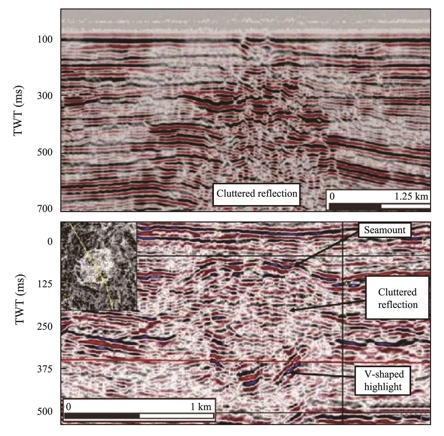
Fig.2 Prediction of shallow gas based on seismic data.

4 Simulation Experiments

4.1 Laboratory Equipment

The experimental equipment is shown in Fig.3 included an experiment rack, pneumatic booster equipment, a high- pressure reactor, and a sonic tester.The experiment rack provided the working area, while the reactor provided a high-pressure sealed environment for the simulation of shal- low gas.The reactor was equipped with a feed port, which can simulate shallow layers by adding sand and injecting gas. It can also change the proportions of sand and gas to alter the porosities and pressure levels of shallow formations. One end of the pneumatic booster was connected withthe gas source, while the other end was connected with the experimental reactor for filling gas.Deep-water shallow soil contains great amounts of media because the deep- water shallow gas-bearing stratum contains high amounts of sand and gas and low amounts of other particles or clay content. Given that the effects of clay and other particles on the speed of sound can be ignored, we decided to esta- blish a simplified model in this work using sand and gas.Furthermore, to achieve different pressures and depths, the pneumatic booster used a small booster pump with a rated boosting capacity of 5MPa and an accuracy of 0.05MPa.The transmitter and transducer were placed on oppo- sitesides at the bottom and top of the simulated formation.The transmitter excited sound waves that traveled through the ground to reach the transducer.The reactor was equip- ped with one transmitter and two transducers.

Compared to predecessors that used airbags for shallow gas experiments, the reactor used in this experiment can withstand greater pressure. Furthermore, the acoustic wave sensor was placed in the reactor, which can avoid the influence of the airbag boundary on the propagation of sound waves. The reactor can be used not only for the simulation of shallow gas but also for the simulation of shallow soil and water flow.

Fig.3 Schematic diagram of the simulation experiment.

4.2 Experimental Program

The longitudinal wave speed in the simulated gas formation was measured using the acoustic measurement sys- tem. To study the changes in longitudinal wave propagation speed, the shallow gas simulation layer volume was fixed by changing the pressure and porosity of the simulated layer. The porosities of the simulated formations wereset as follows: 30%–80% at 10% increments. The specific steps are as follows:

1) Make a simulated shallow gas formation with a certain porosity. Place calculated volumes of sand and gas into the experimental reactor to simulate different formation porosities. The effective porosity expression is shown in Eq. (1) as follows:

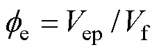
whereeis the effective porosity of the formation, dimensionless;epis the pore volume, cm3; andfis the total vo- lume of the formation, cm3.

2) Seal the reactor so that the soil can freely settle and becomes compacted.

3) Use pneumatic pressurization equipment to inject gas into the reactor. Measure the internal pressures of the formations as 0.1–1.5MPa, with 0.1MPa increments. Seven sets of data should be measured under each pressure condition.

4) Make simulated formations with different formation porosities sequentially and repeat the above steps.

After the experiments, the wave speed must be calculated.Wavelet analysis has advantages in detecting the arrival time of the first arrival wave (Bachman, 1989).The principle of wavelet analysis is based on a time-frequency localization analysis method, in which both the time and the frequency windows can be changed (also known as a ‘mathematical microscope’).When the acoustic signal rea- ches the transducer, the waveform changes suddenly, forming a sudden change point.The wavelet transform coefficient at the mutation point has a modulus maximum. Through multi-scale analysis and modulus maximum detection of acoustic signals,the mutation point can be detected in order to read its time value (., the accurate time value of the first arrival wave). The wavelet transform expressions are given by:

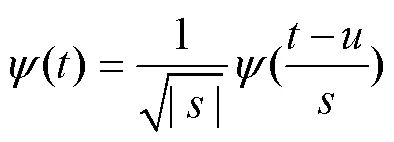
When timeis read by the wavelet transform, this can be combined with the thickness of the simulated formation so that the longitudinal wave speed can be calculated as:

whereVis the longitudinal wave speed,is the thickness of the formation, m; andis the propagation time of the sound wave in the formation, µs.

5 Acoustic Prediction Model of Deep-Water Shallow Gas

The TH206 acoustic wave tester used in this experiment can automatically detect a reasonable waveform and extract the acoustic time difference based on the waveform information to further calculate the acoustic wave speed. One of the waveforms detected in this experiment is shown in Fig.4.

Fig.4 Waveform diagram.

The calculated wave speed value with a large deviation is discarded.The results are shown in Table 1.

The data in Table 1 are fitted with nonlinear binary functions.The graph of the speed change with pressure and po- rosityis shown in Fig.5.

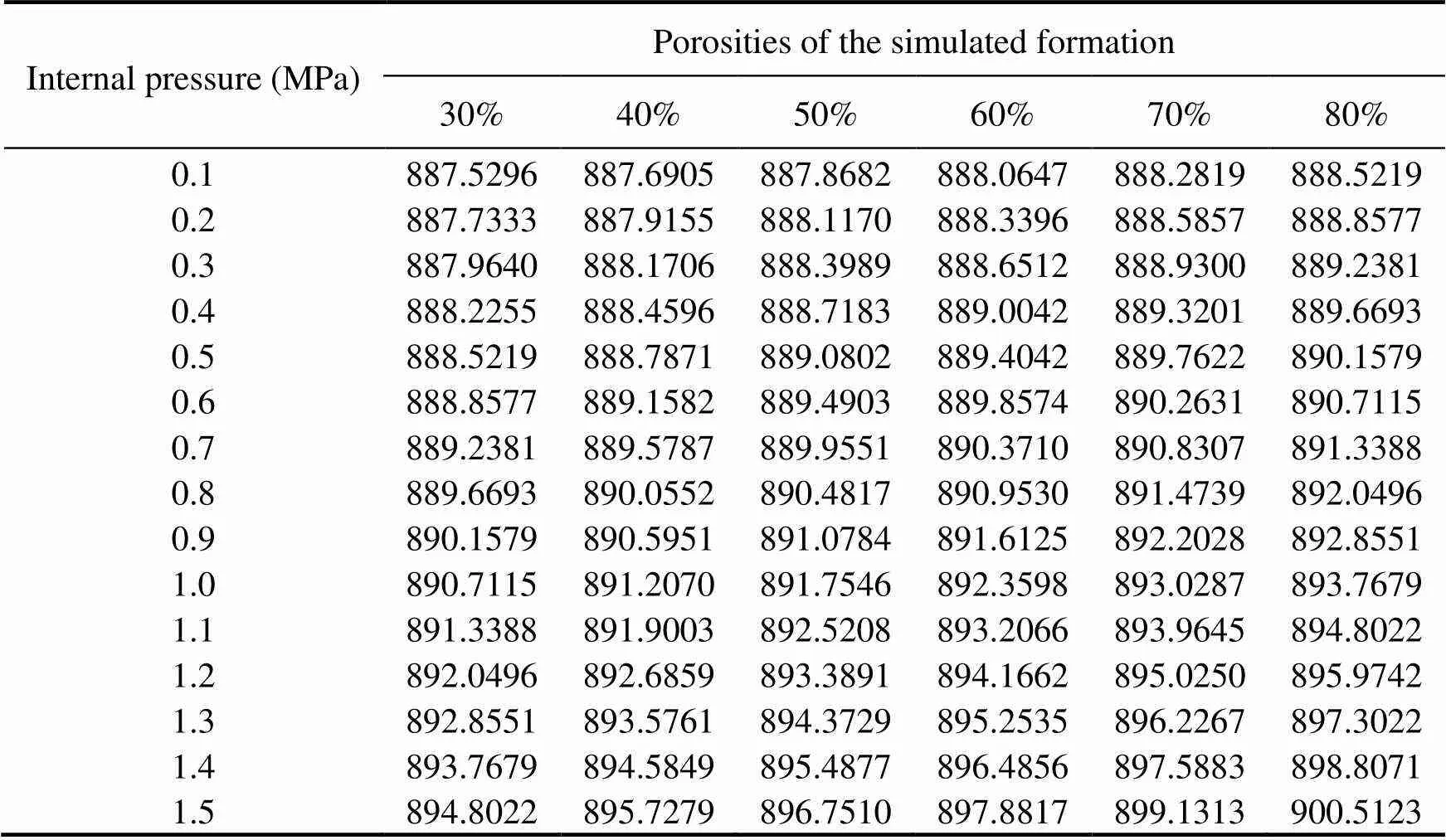
Table 1 The average speeds of sound wave propagations

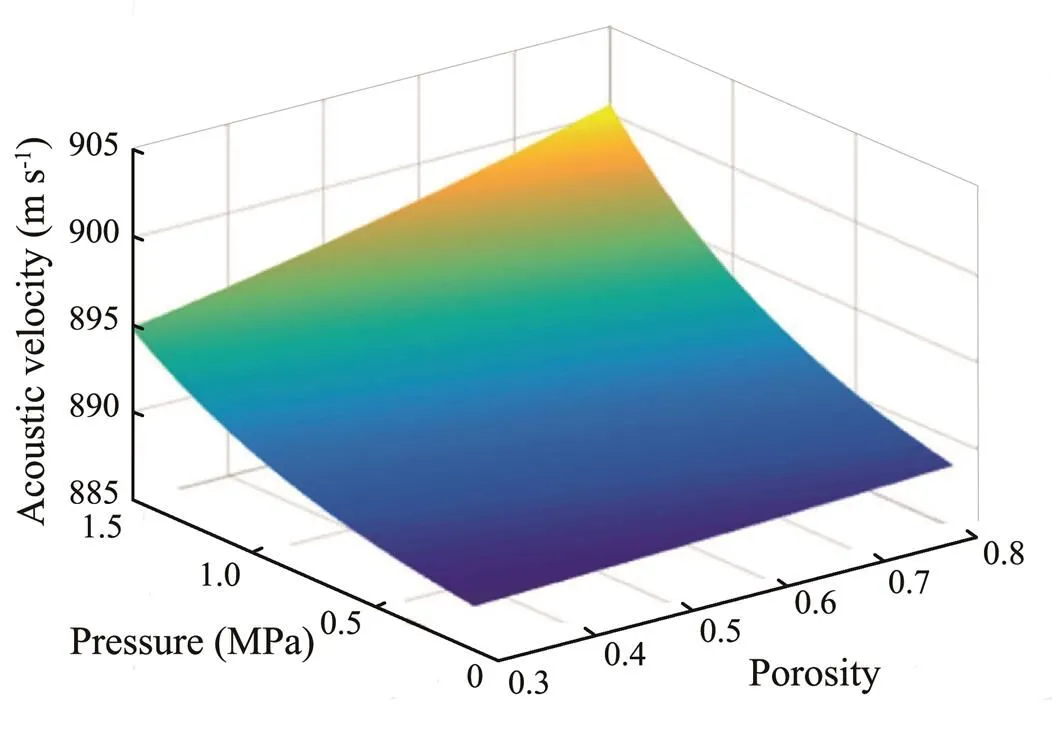
Fig.5 Relationships of acoustic wave propagation speed with porosity and pressure.

As shown in Fig.5, the propagation speed in the shallow gas formation increases with increasing pressure and decreases with increasing porosity. When the pressure is small, the speed increases faster with the pressure, whereas when the pressure is large, the speed increases slowly, in- dicating a power exponential function relationship. The fitting expression is given by:

whereis the sound wave speed, ms−1;ispressure, MPa;is the formation porosity, dimensionless; and1,2, and3are constants related to different regions.When the model is applied to other sea areas, three coefficients must be obtained from the data that have been drilled in the sea area. Thus, the model can be used to predict shallow gas that has not been drilled.

6 Evaluation of Shallow Gas Risks

Once the shallow gas pressure is calculated, the engineering risk can be evaluated. Numerical simulation was adopted in this work to simulate the eruption speed of shal- low gas with different pressures. Here we set the shallowgas reservoir to be located 400m below the mud line, with an area of 2500m2, a water depth of 1000m, a porosity of 0.5, and a permeability of 2500mD, and the corresponding pressure coefficients are 1.05, 1.1, 1.15, and 1.2.The model is presented in Fig.6.

Fig.6 Numerical model of the shallow gas reservoir.

Assuming a thickness of 5m, wecalculated the instantaneous eruption speed levels of shallow gas at different pressure coefficients. The numerical simulation results are shown in Fig.7, while the accumulated total erupted gas volumes are shown in Fig.8.

According to the results, when the formation pressure coefficient is 1.1, the instantaneous eruption speed reachesup to 15m3min−1. After 1h, the cumulative eruption volume reaches 600m3. According to a study (Adams and Kuhl- man, 1990), sand-bearing gas at this speed can cause da- mage to the wellbore. Furthermore, if the formation pressure coefficient increases by 0.05, the instantaneous eruption speed increases close to 5m3min−1. The instantaneous erup- tion speed of shallow gas is more sensitive to the change of pressure. Accordingly,shallow gas pressure coefficients can be defined as low-, medium-, and high-risk if they fall within the ranges of 1.0–1.1, 1.1–1.2, and beyond 1.2, res- pectively.

Fig.7 Instantaneous eruption speed of shallow gas at diffe- rent pressure coefficients.

Fig.8 Accumulated total erupted gas volumes.

Combined with the prediction model, the pressure of shallow gas can be quantitatively determined, and the dril- ling risk level can be evaluated.The specific steps are as follows:

1) Calculate the porosity of the formation.

2) Calculate the speed of sound waves.

3) Assess the shallow gas pressure quantitatively.

4) Assess the drilling risk.

7 Case Study

The water depth of one block in the South China Sea is around 1000m.Before starting drilling, the shallow seismic profile as Fig.9 showed, indicated that there may be shal- low gas at this position. According to the adjacent well data, the porosity at 300m below the mud line is 38%.

Through preliminary exploration of seismic data, we find that the layer velocity at this depth is 915.6901ms−1.By incorporating porosity and speed into Eq. (5), the shallow gas pressure of this layer was calculated to be 13.25MPa, while the pressure coefficient was 1.15, indicating that this layer fell within the medium-risk interval.Therefore, it is recommended that the pilot hole should be drilled, and the dynamic kill technology should be adopted.In the end, the well was successfully completed, during which shallowgas was detected, but due to sufficient preparation work, noeconomic losses were caused, and the shallow gas section was smoothly drilled through.

In addition, the field drilling operation data are basically consistent with the calculated results of the model, indicating the model’s practicability and accuracy when applied to the South China Sea.This model has been used to predict shallow gas in more than 20 wells. Meanwhile, the data of nine typical wells are shown in Table 2.As canbe seen, the prediction accuracy of the model exceeds 90%,., the error between the predicted pressure and the actual pressure is within 10%. The reason for the error may be that the instability of the sound wave measurement leads to a small deviation in the sound velocity measurement. However, this error is within the acceptable range and doesnot affect the safety of drilling. Through literature research and summary analysis of domestic and foreign cases, the accuracy rate is over 90% at a relatively advanced level in the world.

Fig.9 Shallow seismic profile.

Table 2 Results comparison

8 Conclusions

1) The seismic wave propagation speed in the shallow gas formation increases with increasing pressure and decreases with increasing porosity. When the pressure is small,the speed increases faster with the pressure, whereas when the pressure is large, the speed increases slowly, basically showing a power exponential function relationship.

2) The pressure of shallow gas is quantitatively predicted based on the simulation experiment.This method considers the impact of formation porosity on the acoustic speed and can accurately predict shallow gas pressurethrough the logging data of adjacent exploration wells, thus facilitating the evaluation of the drilling risk.

3) Compared to the conventional methods, the method and process established in this paper have realized the tran- sition from qualitative to quantitative prediction of shallow gas. It can quantitatively predict the formation pressureof shallow gas and then take different risk avoidance mea- sures through various pressure coefficients. The prediction method has been applied in the South China Sea. The results indicate that the model has good adaptability with a prediction accuracy of 90%.

Acknowledgements

The study is supported by the National Natural Science Foundation Project ‘Research on the Evolution Mechanism of Bearing Capacity of Deep-Water Oil and Gas WellConduit’ (No. 51774301) and CNOOC Joint Research Project ‘Geotechnical Engineering Parameters Prediction Experiment Based on Acoustic Characteristics of Shallow Layer in the South China Sea’ (No. CCL2020RCPS0120 XNN).

Adams, N. J., and Kuhlman, L. G., 1990. Case history analyses of shallow gas blowouts..Hou- ston, SPE-19917-MS.

Azadpour, M., Manaman, N. S., Kadkhodaie-Ilkhchi, A., and Sedghipour, M. R., 2015. Pore pressure prediction and mo- deling using well-logging data in one of the gas fields in South of Iran., 128: 15-23.

Bachman, R. T., 1989. Estimating velocity ratio in marine sedi- ment., 86 (5): 2029-2032.

Carcione, J. M., and Tinivella, U., 2001. The seismic response to overpressure: A modelling study based on laboratory, well and seismic data., 49 (5): 523-539.

Fleischer, P., Orsi, T., and Richardson, M., 2003. A global survey of the distribution of free gas in marine sediments., 114 (4): 2316- 2317.

Gu, Z. F., Zhang, Z. X., and Wen, Z. H., 2013. Analysis of the distribution characteristics of shallow gas in the northern part of the East China Sea.. Kunming, 94-95.

Hou, Z. Y., Guo, C. S., and Wang, J. Q., 2013. Surface sedimentsacoustic speed and porosity correlation in Nansha sea areaabyssal region., 37 (7): 77-82 (in Chinese with English abstract).

Kraft, B. J., Mayer, L. A., Simpkin, P., Lavoie, P., Jabs, E., Lyns- key, E.,., 2002. Calculation ofacoustic wave pro- perties in marine sediments. In:. Pace, N. G., and Jensen, F. B., eds., Springer, Dordre- cht, 123-130.

Long, J. J., and Li, G. X., 2015. Theoretical relations between sound velocity and physical-mechanical properties for seafloor sediments., 40 (3): 462-468 (in Chinese with English abstract).

Mayer, L. A., Kraft, B. J., Simpkin, P., Lavoie, P., Jabs, E., and Lynskey, E., 2002.determination of the variability of seafloor acoustic properties: An example from the ONR geoclutter area. In:. Pace, N. G., and Jensen, F. B., eds., Springer, Dordrecht, 115-122.

Savvides, C., Tam, V., Os, J. E., Hansen, O., van Wingerden, K., and Renoult, J., 2001. Dispersion of fuel in offshore modules: Comparison of predictions using FLACS and full-scale experiments.. ERA, ISBN0700807489.

Wang, H. H., Yang, J., Li, L., Xu, J. J., Meng, L. Y., Hong, J. J.,., 2019. An acoustic approach to identify shallow gas and evaluate drilling risk in deep water based on simulation experiment study.. Honolulu, ISOPE-I-19-601.

Weber, M. E., Niessen, F., Kuhn, G., and Wiedicke, M., 1997. Calibration and application of marine sedimentary physical properties using a multi-sensor core logger., 136 (3-4): 151-172.

Yang, J., Zhang, B. L., Zhou, B., Xu, P., and Tian, R. R., 2015. Geological disaster acoustic wave identification and prediction technology of deepwater shallow gas., 37 (1): 143-146 (in Chinese with English abstract).

Zou, D. P., Wu, B. H., and Lu, B., 2007. A research on error analysis of seabed sediment porosity by calculation method andsonic speed retrieval method.,26 (4): 32-36.

October 9, 2020;

November 15, 2021;

December 30, 2021

© Ocean University of China, Science Press and Springer-Verlag GmbH Germany 2022

. Tel: 0086-10-84526251

E-mail: tonggang@cnooc.com.cn

(Edited by Chen Wenwen)