DUAN Chenglin, WANG Zhifeng, and DONG Sheng

Intensity of Level Ice Simulated with the CICE Model for Oil-Gas Exploitation in the Southern Kara Sea, Arctic

DUAN Chenglin, WANG Zhifeng, and DONG Sheng*

College of Engineering, Ocean University of China, Qingdao 266100, China

Sea ice is the predominant natural threat to marine structures and oil-gas exploitation in the Arctic. However, for ice-resistant structural design, long-term successive level ice thickness measurements are still lacking. To fill this gap in the southern Kara Sea, the Los Alamos Sea Ice Model (CICE) is applied to achieve better simulation at the local and regional scales. Based on the validation against ice thickness observations in March and April in 1980–1986, the statistical root-mean-square error is determined to be less than 0.2m. Then, based on the hindcast data, the spatiotemporal distributions of level ice thickness are analyzed annually, seasonally, and monthly, with thicker level ice of 1.2–1.5m in spring and large ice-free zones in September and October. For floating platforms, a novel ice grade criterion with five classifications, namely, excellent, good, moderate, severe, and catastrophic, is proposed. The first two grades are most suitable for offshore activities, particularly from August to October, and the moderate grade is acceptable if with ice-resistant protections. Furthermore, hostile ice conditions are discussed in terms of the generalized extreme value distribution. The statistics reveal that at a return period of 100yr, extreme level ice is primarily between 0.6m and 1.0m in December. The present investigation could be a useful reference for a feasibility study of the potential risk analysis and ice-resistant operation of oil-gas exploitation in the Arctic.

level ice; CICE; spatiotemporal distribution; return period; ice-resistant floating platform; southern Kara Sea

1 Introduction

The Arctic is believed to be the region with the most abundant undiscovered hydrocarbon deposit in the world. Even though the Arctic encompasses only 6% of the Earth’s surface, 30% of unexplored gas and 13% of unex- plored oil can be found there, particularly in the Russian Arctic (Gautier., 2009). However, this cold area has extreme oceanic environmental conditions, such as low temperature, long polar nights, polar lows, dense fog, and extensive ice and snow cover. In particular, the formation of sea ice can not only influence the marine environment, atmospheric circulation, and climate change (, Budi- kova, 2009; Mori., 2014; Zhao., 2019), but also threaten shipping navigation, drilling platform operation, and other marine activities (, Timco and Weeks, 2010; Marchenko, 2014; Gudmestad, 2018).

The southern Kara Sea (SKS) is a semi-closed shelf sea and contains 39% potential oil-gas resources, ranking first in the Russian Arctic. As shown in Figs.1 and 2, the SKS is surrounded by different lands and seas, with the west separated from the Barents Sea by Novaya Zemlya, the south and east bounded by the Eurasian continent, and the north connected to the northern Kara Sea by the boundary (denoted by the dotted line at the center) between Cape Zhelaniya and Dikson Island. The bathymetry is also favorable to oil-gas exploitation in terms of the average depthof 110m, with 40% less than 50m. In a Russian plan, 60% of oil-gas production in 2035 is expected from the SKS fields (Bekker., 2015). In general, sea ice is the predominant natural threat to oil-gas exploitation and marine structures in the Arctic. Thus, spatiotemporal analysis and intensity assessment of sea ice conditions in the SKS have become important research topics.

In general, sea ice is an inevitable challenge to oil-gas exploitation in the SKS (Efimov., 2020). Different from the western Barents Sea, which is toward an ice-free zone even in the winter months (Onarheim and Årthun, 2017; Duan., 2018), the fixed offshore platform can operate all year round without ice threats. Subjected to the blocking effect of Novaya Zemlya, large amounts of North Atlantic warm waters cannot freely enter the SKS (Duan., 2019). Thus, the SKS maintains longer cold and frozen conditions. Ice-free periods are limited to 2–3 months on average and have prominent interannual variability (Duan., 2019; Efimov., 2020). In this seasonally ice-covered area, the mobile floating platform is a feasible choice (see Fig.2). In open waters, the mobile floating platform can operate safely; in light ice conditions, it can still work with the protection of ice-resistant structures, such as shockproof walls; and in the case of hazardous ice loads, it can be promptly disconnected and evacuated from the drilling site (Kutvitskaya and Ryazanov, 2013).

Fig.1 Location and bathymetry of the southern Kara Sea.

At present, the regulations for polar sea ice engineering in China are still incomplete. Therefore, the determination of the intensity of sea ice for the design and operation of ice-resistant floating platforms in the SKS requires com- prehensive knowledge. Level ice thickness needs to be de- termined and carefully considered. The mechanical prop- erties of ice and their associated theoretical formulas are closely dependent on their physical properties, such as compressive and flexural strength (Timco and Weeks, 2010; Kovalev., 2019; Chai, 2021). However, most relevant investigations concentrated primarily on the spatiotemporal sea ice extent trends and their associated relationship with metocean factors in the SKS (, Belchansky., 1995; Divine., 2004; Rodrigues, 2008; Zubakin., 2008; Cavalieri and Parkinson, 2012; Ahn, 2014; Matishov., 2014; Bushuk and Giannakis, 2017; Duan., 2019, 2020; Efimov., 2020). Few studies have emphasized the sea ice thickness distributions across the SKS because of the scarcity of long-term successive level ice thickness observations.

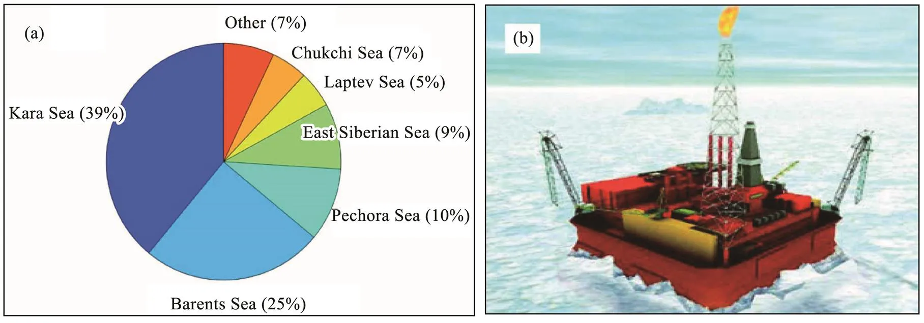
Fig.2 Oil-gas proportional distributions in the Russian Arctic (a) and floating drilling platform (b). The statistical data were obtained from Wang (2017), and the platform picture was taken from Karulin and Karulina (2010).

Generally, several methods can be possibly used to determine ice thickness in the Arctic. 1) Drilling holes is the most accurate approach, as demonstrated in the fieldwork conducted by Romanov (2004) and Kovalev. (2019). 2) Airborne electromagnetic observation is an efficient, fast, and high-precision method that has been successfully used to measure the pack sea ice areas in March and April (Haas., 2010). 3) Subsea upward-looking sonar can obtain measurements over relatively long distances (Birch., 2000). However, these three methods require considerable labor and material costs and are often limited to strict geopolitics. Furthermore, the observations usually vary by region at different times of the year, making it impossible to convert the scattered data into an area-averaged spatial ice thickness picture. 4) Satellite monitoring: Since 2002, with the launch of ENVISAT, CryoSat-2, and SMOS satellites, large grid-scale winter ice thickness can be determined using remote sensing technology. However, the retrievable data show possible uncertainties and are easily contaminated by the poor atmospheric environment (Huntemann., 2014; Ricker, 2014). 5) Stefan’s empirical formula: In this hypothesis, the level ice thickness is assumed to be proportional to the square root of the sumof freezing degree days (Ashton, 1986). This equation only considers the air temperature over the sea surface, not the sea ice dynamics.

To overcome the aforementioned defects, numerical sim- ulation is another effective and powerful technology used to reproduce the historical sea ice freezing–melting processes and fill the gap of long-term successive level ice thickness in the SKS. A short-term attempt during the winter of 2008–2009 was conducted in several coastal sites using the thermodynamic sea ice model HIGHTSI (Cheng., 2013; Similä., 2013), but it did not examine the ice thickness spatial pattern across the SKS. Some reanal- ysis data, such as TOPAZ4, PIOMAS, ORAP5, ORAS5, CFSR, and CFSv2, have been available. The TOPAZ4 pro- duct was well assessed (Xie, 2017) and even recommended for the medium-range predictability of early sum- mer sea ice thickness distribution in the East Siberian Sea (Nakanowatari, 2018). However, the TOPAZ4 product did not assimilate sea ice thickness from the CryoSat-2 and SMOS satellite until 2014. No reliable conclusions on sea ice thickness in the SKS were obtained because no direct comparison withobservations, particularly in periods without assimilation, was conducted. Moreover, the Los Alamos Sea Ice Model (CICE) (Hunke, 2015), which integrates the complete sea ice physical theories and parameterizations, has been widely applied to conduct sci- entific studies of Arctic sea ice (Wu, 2015). The CICEprovides three types of thermodynamics,, zero-layer module (Semtner, 1976), Bitz-Lipscomb module (Maykut and Untersteiner, 1971; Lipscomb, 1998; Bitz and Lips- comb, 1999), and mushy module (Feltham., 2006), and two types of dynamics,, elastic-viscous-plastic (EVP) module (Hunke, 2001; Hunke and Dukowicz, 1997, 2002, 2003; Bouillon., 2013) and elastic-anisotrop- ic-plastic (EAP) module (Wilchinsky and Feltham, 2006; Tsamados., 2013). In general, most studies show that the simulated sea ice extent interannual variability coincides well with the satellite observations in the Arctic. However, the simulation performance is primarily evaluated on a large global scale (, regarding the central Arctic and all of the marginal seas as a unified whole) and focuses mainly on the ice extent rather than the ice thickness (, Hunke and Bitz, 2009; Flocco., 2012;Wang and Su, 2015; Wu, 2015; Urrego-Blanco., 2016; Chu., 2019). Few studies have explored the simulation capability on the regional and local scales (, separate marginal seas, such as the Kara Sea and the Laptev Sea). Different thermodynamic coupling selections with different physical parameter sets canresultinsignificantdifferencesinthesimulation(Hunke,2010; Wu, 2015; Urrego-Blanco., 2016). Therefore, in marginal and regional seas, such as the SKS, the local model configuration should be thoroughly tested, given that we particularly emphasize the intensity of level ice thickness for ice-resistant offshore structures.

This study constitutes the first quantification of the level ice thickness and associated concept on ice-resistant float- ing platforms across the SKS. Three critical topics are studied. First, we quantitatively explore configurations in the CICE model to achieve better ice simulation at the local SKS scale. Second, we supplement a 30-year level ice thickness database from 1980 to 2009 and determine its spatiotemporal characteristics. Third, for floating plat- form design and operation, we propose a reasonable ice regime grade classification criterion and estimate hostile ice conditions at longer return periods based on extreme value statistics. We hope that the present work could be a useful reference for a feasibility study of the potential oil-gas exploitation and ice-resistant structural design in the SKS, particularly for researchers with considerable interests in the Arctic but are far from it geographically.

2 CICE Model Setup and Validation

2.1 Ice Thickness Distribution (ITD) Function in the CICE

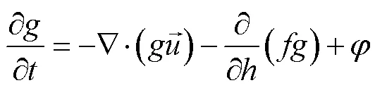
The CICE defines an ITD function=(,,) to simulate the sea ice pack evolution in time and space. In this function,=(,) denotes the ocean surface grid,denotes the longitude,denotes the latitude,denotes the time, anddenotes the ice thickness. At a given time and location,(,,)dis the fractional area covered by ice in the thickness range [,+d]. Thus, the ITD function is numerically regarded as the approximation of the basic thickness evolution (Thorndike, 1975), which can be expressed as follows:

To solve Eq. (1), the CICE discretizes the ice pack into different thickness categories in each grid cell. The number of categoriescan vary from 1 to 15, with the upper boundaryHfor each categorydetermined using the following recursive equation (Lipscomb, 2001):

with0=0,1=3/,2=151, and3=3.

2.2 Model Configuration

Sea ice evolution processes are closely dependent on the metocean conditions. Based on previous research (Wang and Su, 2015; Wu, 2015; Wang, 2020), the following meteorological and oceanographic forcing fields are selected to achieve better simulation performance in the SKS. For atmospheric conditions, the sea air temperature, wind, specific humidity, and precipitation are obtained from the Common Ocean Reference Experiments version 2 dataset (Griffies, 2009), whereas the cloud fraction is obtained from the Arctic Ocean Model Intercomparison Project dataset (Hunke and Holland, 2007). For oceanic conditions, the sea surface tilt, current, and thermal flux are obtained from the Community Climate System Model climate dataset (Collins, 2006), where- as the sea surface salinity and temperature are obtained from the Polar Science Center Hydrographic Climatology version 3.0 dataset (Steele, 2001; Wang and Su, 2015).

The present simulation is conducted based on the inherent gx1 displaced pole grids in the CICE. Five categories of ice thickness, namely, 0–0.64, 0.64–1.39, 1.39–2.47, 2.47–4.57, and >4.57m, are selected (Hunke and Bitz, 2009). The EVP dynamics and mushy thermodynamics are coupled. Moreover, the bubbly brine algorithm for thermal conductivity, linear remapping scheme for advection, and Delta-Eddington method for shortwave are selected. Table 1 lists the primary inputted run parameters. The sea air temperature, specific humidity, precipitation, cloud fraction, thermal flux, sea surface salinity, and temperature are inputted into the mushy thermodynamics mod- ule, whereas the wind, current, and sea surface tilt are inputted into the EVP dynamics module. The initial condition is set as a cold start with no ice, given the lack of data. To achieve better model stability, the total run duration is from January 1969 to December 2009 with a 1-h time step. For the ice-resistant design of floating platforms, assessments of the modeled level ice thickness during 1980–2009 in the SKS are emphasized (Fig.1).

Table 1 Primary setup of thermodynamics and dynamics in our CICE simulation

Note: Other parameters are used with default options.

2.2 Model Validation

Verification analysis is performed between simulated level ice thickness and scattered observations in the SKS. Themeasurement data are obtained from the Soviet Union’s historical Sever airborne and North Pole drifting station program (Borodachev and Shilnikov, 2002; Romanov, 2004). During this program, the level ice thickness was discretely measured by drilling ice holes on the aircraft runway in the Russian Arctic, where the sea ice cover was completely frozen in March, April, and May from 1928 to 1989. First, the age and partial concentration of ice were determined using low-flying aircraft. After landing, three to five measurements of thickness at 150–200m intervals were made on the runway. Then, the values were averaged and regarded as the level ice thickness in this location. Thus, one data record exists for each location. Herein, data during 1980–1986 in the SKS were selected. Fig.3 shows these scatteredlocations in March and April. Each location denotes one valid measurement. For comparison, the simulated data were gridded into the observed scattered locations in time and space by applying a bilinear interpolation.

Fig.4 illustrates the comparison between drilled and simulated level ice thicknesses in March and April. The results indicate the good consistency between both data. The bias, mean absolute error, and root-mean-square error (RMSE) are relatively small, whereas Pearson’s correlation coefficient () can be up to 0.80 and 0.76. Therefore, the simulated level ice thicknesses in these locations are acceptable, and we deduce that the spatiotemporal variations of level ice thickness in the SKS could be approximately reproduced well based on the present CICE configuration. However, the simulation results for April are somewhat higher than the observations. We infer that the simulated thicker sea ice is largely caused by the inputted overestimated low sea air temperatures or underestimated inflowing heat in the thermal flux. However, because of the lack of measured hydrometeorological data in the Arctic region, the reanalysis data for forcing fields in the present CICE run were not fully assimilated to reduce these deviations. Thus, to decrease the inconsistencies be- tween simulations and observations, both the more accurate inputted metocean forcing data and reasonable sea ice parameterizations of the model should be thoroughly explored.

Fig.3 Overview of the discrete ice thickness observations in March and April. The red circles and triangles are the locations, and the associated black numbers represent the time of measurement.

Fig.4 Validations between simulated and observed level ice thicknesses in March and April. In (b), the index used in the x-axis corresponds to the spatial and temporal variabilities in Fig.3.

3 Spatiotemporal Variation of Level Ice

3.1 Annual Distribution of Level Ice Thickness

The 30-year hindcast data during 1980–2009 in the CICE model are selected to determine the mean annual distribution of level ice thickness in the SKS. This spatial pattern is illustrated in Fig.5.

Fig.5 Annual distribution of the mean level ice thickness in the southern Kara Sea.

As shown in Fig.5, the total domain is covered by level ice with varying thickness. In general, the mean annual level ice thickness primarily ranges from 0.5m to 1.0m across the SKS. The thinnest level ice (<0.6m) is primarily distributed in the southern zone, the median (0.7–0.8m) is primarily distributed in the central zone, and the thickest level ice (>0.9m) is primarily distributed in the northwest zone. Moreover, a relatively thinner zone (<0.7m) is observed in the eastern estuary adjacent zone. Overall, the level ice gradually becomes thicker from southwest to northeast with the increasing latitude.

3.2 Seasonal Distribution of Level Ice Thickness

The seasonal mean spatial distributions of the level ice thickness are also analyzed herein. Considering the spatiotemporal characteristics of the ice cover in the Kara Sea (Duan., 2019), in this study, January-February-March is defined as winter, April-May-June is defined as spring, July-August-September is defined as summer, and October-November-December is defined as autumn. These seasonal patterns are shown in Fig.6.

As shown in Fig.6, the four seasons exhibit different level ice thicknesses in the SKS. In spring, the level ice is the thickest,, primarily between 1.1m and 1.5m from south to north. In winter, the level ice is the second thickest,, mainly between 0.7m and 1.4m. In autumn, the level ice thickness is no more than 0.4m. In summer, the SKS has the relatively thinnest level ice thickness of less than 0.3m in most regions. Thus, the level ice thickness has an obvious seasonal variation in the SKS.

3.3 Monthly Distribution of Level Ice Thickness

The monthly distribution analysis is informative and in-dispensable to floating platform design suitable for oil-gas exploitation and can directly determine the operation dura- tion and ice-resistant requirements. The simulation results show that level ice thickness has a typical increasing-de- creasing cycle and a noticeable monthly variation in the SKS, indicating that monthly sea ice tends to be 1-year level ice.

In detail, Fig.7 plots the contours of the monthly spatial patterns of the mean level ice thickness in the SKS from January to December. In terms of the temporal variability, the entire domain is covered with thicker level ice in the winter and spring months, whereas large ice-free zones occur in the SKS in the summer and autumn months. The level ice approaches the thickest,, primarily between 1.2m and 1.5m, in May. In April, June, and March, the level ice exceeds 1m in most areas. February and January are the two other months that have relatively thicker level ice,, between 0.6m and 1.0m. Meanwhile, July with level ice thickness of 0.6m is the transitional month when ice begins to break up. In August, the thickness even decreases to 0.1m. Things are quite different in September and October. During both months, the SKS is characterized by large open waters. Then, in November, seawater refreezes again but cannot form 0.4m level ice thickness. In December, the level ice thickness mainly varies from 0.3m to 0.7m. The monthly variations of the simulated level ice thickness in the present CICE configuration also exhibit good consistency with the calculated values from an earlier thermohaline and ice model established by the Eco-System Company during 1990–1995 (Arhipov., 1996). In this model, the maximum level ice thickness was equal to the observed 1.4m in May at Baidara Bay, which is located on the southeastern part of the SKS. Therefore, we can conclude that September and October are the two optimal months for oil-gas exploitationwithout severe ice threats. To improve economic efficiency, floating platform operations may be extended in several ice-covered months.

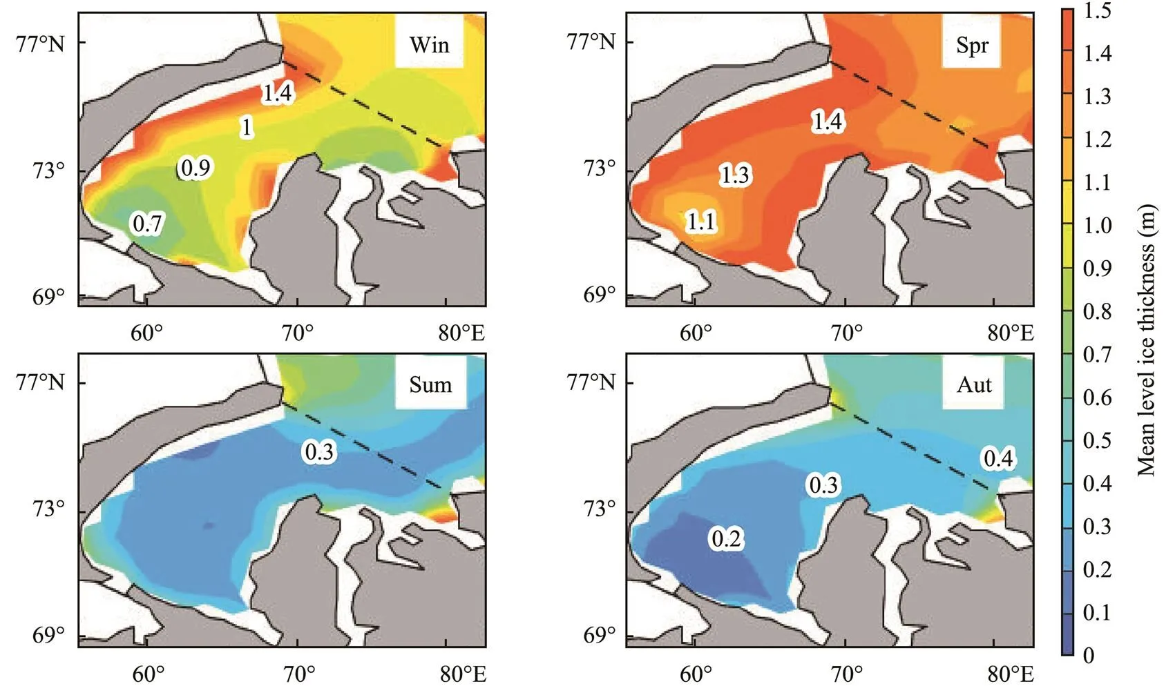
Fig.6 Seasonal distribution of the mean level ice thickness in the southern Kara Sea.

Fig.7 Monthly distribution of the mean level ice thickness in the southern Kara Sea.

4 Grade Divisions and Extreme Ice Conditions

4.1 Grade Divisions of Level Ice

Based on the monthly distribution analysis, 1-year levelice can be up to 1.5m in the SKS. The World Meteorological Organization (WMO, 1985) categorizes the climatologic ice types according to the ice formation and development stages as follows:

1) Nilas ice, with an ice thickness of less than 0.1m;

2) Young ice, with an ice thickness of 0.1–0.3m;

3) Thin ice, with an ice thickness of 0.3–0.7m;

4) Medium ice, with an ice thickness of 0.7–1.2m;

5) Thick ice, with an ice thickness of more than 1.2m.

The ISO 19906 code (International Organization for Standardization, 2010) also employs this classification criterion (hereafter WMO criterion) for the Arctic 1-year level ice. Thus, based on this grade division method, level ice types in each month across the SKS can be summarized as shown in Table 2. These results are acceptable for climatologic analysis. However, this grade division method does not completely consider the engineering characteristics of the floating platform, such as the installation, operation, movability, and associated oil-gas transportation and storage. Therefore, by combining the WMO criterion with the spatiotemporal ice concentrations (Duan., 2019), we propose a more reasonable grade division method of level ice for floating platforms in the SKS. As shown in Table 3, ice condition grades are categorized into five groups, namely, excellent, good, moderate, severe, and catastrophic. For floating platforms in the SKS, the first two grades are best, the moderate grade is acceptable if with good ice-resistant protections, and the last two grades are deemed as threatening and disastrous cases.

Table 2 Monthly ice types in the SKS based on the WMO criterion

Table 3 Proposed monthly grade division of level ice condition

4.2 Extremal Analysis Method

Floating platforms and other marine structures may suffer from extreme sea ice loads but should survive. Thus, extreme ice conditions at longer return periods must be predicted. In engineering practice, one can fit the extreme value distribution function to a set of maxima derived from subsets of the sample data (, daily, monthly, seasonal, annual maxima) (Coles, 2001). Several mathematical modeling functions, such as Gumbel (Type I), Fréchet (Type II), and Weibull (Type III), have been considered. Theoretically, these three distributions are special cases of the generalized extreme value (GEV) distribution (, Coles, 2001).

The cumulative GEV function can be expressed as follows:

where,, anddenote the location, scale, and shape parameters, respectively. Herein, the maximum likelihood is utilized to estimate these three parameters. The corresponding equations can be expressed as follows:

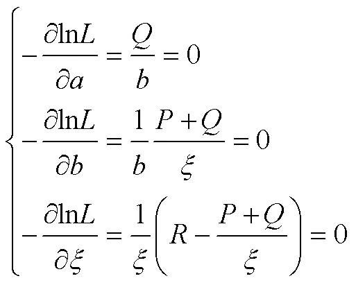
and

where 1ndenotes the likelihood function and (1,1), (2,2),···, (x,y) denote the level ice thickness samples. These equations can be solved by numerical iterations. With the obtained values of,, and, the extreme level ice thickness higher than the observed maxima can be estimated.

4.3 Hostile Ice Condition Estimation

Using the aforementioned grade division method, the extreme level ice thicknesses in November and December across the SKS are estimated based on the monthly maxima of the 30-year simulated ice database.

Fig.8 plots the contours of the spatial patterns of the extreme conditions (, 25, 50, and 100yr) for level ice thickness in the SKS in November and December. The contours seem to have similar patterns but have different values. Regarding the 25yr case, level ice thickness primarily ranges from 0.2m to 0.6m in November and from 0.5m to 0.8m in December. Regarding the 50yr case, level ice thickness mainly ranges from 0.3m to 0.6m in November and from 0.5m to 0.9m in December. Regarding the 100yr case, level ice thickness predominantly ranges from 0.4m to 0.7m in November and from 0.6m to 1.0m in December. Specifically, the level ice thickness at a return period of 100yr can be classified as severe. This hostile ice regime analysis could be a reference for the ice-resistant design of floating platforms and affiliated marine structures in the SKS.

Fig.8 Contours of the extreme level ice thickness in the southern Kara Sea in November and December.

5 Conclusions and Future Work

Floating platforms are suitable for oil-gas exploitation in the seasonally ice-covered SKS. However, long-term successive level ice thickness measurements across the entire SKS are still lacking. To fill this gap, the thermodynamic CICE model coupling the EVP and mushy modules is established at the local SKS scale for the first time. Compared with the available measurements in March and April in 1980–1986, the RMSE of simulated level ice thickness is no more than 0.2m. Based on the hindcast data, the spatiotemporal variations of level ice thickness are analyzed annually, seasonally, and monthly. In general, the ice regime belongs to the 1-year level ice and shows an obvious monthly cycle. Thicker level ice appears during the spring months (thickest in May,, between 1.2m and 1.5m), whereas large ice-free zones occur in September and October. For floating platforms, a new ice grade criterion with five classifications, namely, excellent, good, moderate, severe, and catastrophic, is proposed. The first two grades are optimal for offshore activities, particularly from August to October, and the moderate grade is acceptable if with ice-resistant protections. Furthermore, hostile ice conditions are estimated based on the GEV distribution. At a return period of 100yr, level ice is primarily from 0.6m to 1.0m in December.

The present investigation could be a useful reference for a feasibility study of the oil-gas exploitation and ice-resistant structural design in the SKS. Furthermore, the sea ice engineering characteristics, such as ridges or bergy bits, should be considered. These ice features threaten the safety of Arctic offshore structures. The CICE model can simulate the sea ice ridging process. Regrettably, the currently available field data cannot adequately and reliably validate the simulated ridged ice thickness across the entire SKS. More fieldwork should be conducted in the future.

Acknowledgements

The study is supported by the National Key Research and Development Program of China (No. 2016YFC0303401), the National Natural Science Foundation of China (No. 51779236), and the National Natural Science Foundation of China–Shandong Joint Fund (No. U1706226).

Ahn, J., Hong, S., Cho, J., Lee, Y. W., and Lee, H., 2014. Statistical modeling of sea ice concentration using satellite imagery and climate reanalysis data in the Barents and Kara Seas, 1979–2012., 6 (6): 5520-5540.

Arhipov, B. V., Solbakov, V. V., and Tsvetsinsky, A. S., 1996. Hydrodynamic and ice model or the south-western part of the Kara Sea.. Los Angeles, California, ISOPE-I-96-153.

Ashton, G. D., 1986.. Water Resources Publication, Highlands Ranch, Colorado, 57-60.

Bekker, A. T., Sabodash, O. A., Shpagin, K. D., and Krikunova, Y. A., 2015. Analysis of technical solutions of exploration platforms in shallow waters for the Russian Arctic.. Kona, Hawaii, ISOPE-I-15-195.

Belchansky, G. I., Mordvintsev, I. N., Ovchinnikov, G. K., and Douglas, D. C., 1995. Assessing trends in Arctic sea-ice distribution in the Barents and Kara Seas using the Kosmos-Okean satellite series., 31 (177): 129-134.

Birch, R., Fissel, D., Melling, H., Vaudrey, K., Lamb, W., Schaudt,K.,, 2000. Ice-profiling sonar upward looking sonar provides over-winter records of ice thickness and ice keel depths off Sakhalin Island, Russia., 41 (8): 48-54.

Bitz, C. M., and Lipscomb, W. H., 1999. An energy-conserving thermodynamic model of sea ice., 104 (C7): 15669-15678.

Borodachev, B. E., and Shilnikov, V. I., 2002.Gidrometeoizdat Publishing House, St. Petersburg, 441pp (in Russian).

Bouillon, S., Fichefet, T., Legat, V., and Madec, G., 2013. The elastic-viscous-plastic method revisited., 71: 2-12.

Budikova, D., 2009. Role of Arctic sea ice in global atmospheric circulation: A review., 68 (3): 149-163.

Bushuk, M., and Giannakis, D., 2017. The seasonality and interannual variability of Arctic sea ice reemergence., 30 (12): 4657-4676.

Cavalieri, D. J., and Parkinso, C. L., 2012. Arctic sea ice variability and trends, 1979–2010., 6 (4): 881-889.

Chai, W., Leira, B. J., Høyland, K. V., Sinsabvarodom, C., and Yu, Z., 2021. Statistics of thickness and strength of first-year ice along the northern sea route., 26 (2): 331-343.

Cheng, B., Mäkynen, M., Similä, M., Rontu, L., and Vihma, T., 2013. Modelling snow and ice thickness in the coastal Kara Sea, Russian Arctic., 54 (62): 105-113.

Chu, M., Shi, X., Fang, Y., Zhang, L., Wu, T., and Zhou, B., 2019. Impacts of SIS and CICE as sea ice components in BCC_CSMon the simulation of the Arctic climate., 18 (3): 553-562.

Coles, S., 2001.. Springer, London, 45-72.

Collins, W. D., Bitz, C. M., Blackmon, M. L., Bonan, G. B., Bretherton, C. S., Carton, J. A.,, 2006. The community climate system model version 3 (CCSM3)., 19 (11): 2122-2143.

Divine, D. V., Korsnes, R., and Makshtas, A. P., 2004. Temporal and spatial variation of shore-fast ice in the Kara Sea., 24 (15): 1717-1736.

Duan, C., Dong, S., and Wang, Z., 2020. Mathematical modeling of Arctic sea ice freezing and melting based on nonlinear growth theory., 210: 104278.

Duan, C., Dong, S., Wang, Z., and Tao, S., 2018. Variability Characteristics of winter sea ice in the Barents Sea based on a statistical approach.. Sapporo, ISOPE-I-18-146.

Duan, C., Dong, S., Xie, Z., and Wang, Z., 2019. Temporal variability and trends of sea ice in the Kara Sea and their relationship with atmospheric factors., 20: 136-147.

Efimov, Y. O., Kornishin, K. A., Sochnev, O. Y., Mironov, Y. U., and Porubaev, V. S., 2020. Evaluation of exploration drilling scenarios in the southwestern part of the Kara Sea.. Virtual, ISOPE-I-20-1272.

Feltham, D. L., Untersteiner, N., Wettlaufer, J. S., and Worster, M. G., 2006. Sea ice is a mushy layer., 33 (14): L14501.

Flocco, D., Schroeder, D., Feltham, D. L., and Hunke, E. C., 2012. Impact of melt ponds on Arctic sea ice simulations from 1990 to 2007., 117 (C9): C09032.

Gautier, D. L., Bird, K. J., Charpentier, R. R., Grantz, A., Houseknecht, D. W., Klett, T. R.,, 2009. Assessment of undiscovered oil and gas in the Arctic., 324 (5931): 1175-1179.

Griffies, S. M., Biastoch, A., Böning, C., Bryan, F., Danabasoglu, G., Chassignet, E. P.,, 2009. Coordinated ocean-ice reference experiments (COREs)., 26 (1-2): 1-46.

Gudmestad, O. T., 2018. Technological challenges for sustainable use of the Arctic Seas., 28 (4): 337-341.

Haas, C., Hendricks, S., Eicken, H., and Herber, A., 2010. Synoptic airborne thickness surveys reveal state of Arctic sea ice cover., 37 (9): L09501.

Hunke, E. C., 2001. Viscous-plastic sea ice dynamics with the EVP model: Linearization issues., 170 (1): 18-38.

Hunke, E. C., 2010. Thickness sensitivities in the CICE sea ice model., 34 (3-4): 137-149.

Hunke, E. C., and Bitz, C. M., 2009. Age characteristics in a multidecadal Arctic sea ice simulation., 114 (C8): C08013.

Hunke, E. C., and Dukowicz, J. K., 1997. An elastic-viscous-plastic model for sea ice dynamics., 27 (9): 1849-1867.

Hunke, E. C., and Dukowicz, J. K., 2002. The elastic-viscous-plastic sea ice dynamics model in general orthogonal curvilinear coordinates on a sphere–Incorporation of metric terms., 130 (7): 1848-1865.

Hunke, E. C., and Dukowicz, J. K., 2003. The sea ice momentum equation in the free drift regime. Technical report LA-UR-03-2219. Los Alamos National Laboratory, Los Alamos, New Mexico, 50-55.

Hunke, E. C., and Holland, M. M., 2007. Global atmospheric forcing data for Arctic ice-ocean modeling., 112 (C4): C04S14.

Hunke, E. C., Lipscomb, W. H., Turner, A. K., Jeffery, N., and Elliott, S., 2015.. Los Alamos, New Mexico, USA.

Huntemann, M., Heygster, G., Kaleschke, L., Krumpen, T., Mä- kynen, M., and Drusch, M., 2014. Empirical sea ice thickness retrieval during the freeze-up period from SMOS high incident angle observations., 8: 439-451.

International Organization for Standardization, 2010. ISO 19906: 2010, petroleum and natural gas industries–Arctic offshore structures. International Standardization for Organization, 139-140.

Karulin, E. B., and Karulina, M. M., 2010. Performance studies for technological complex platform ‘Prirazlomnaya’–Moored tanker in ice conditions.. Busan, ISOPE-P-10-005.

Kovalev, S. M., Smirnov, V. N., Borodkin, V. A., Shushlebin, A. I., Kolabutin, N. V., Kornishin, K. A.,, 2019. Physical and mechanical characteristics of sea ice in the Kara and Laptev Seas., 29 (4): 369-374.

Kutvitskaya, N. B., and Ryazanov, A. V., 2013. Engineering protection for permanent offshore platform against ice impact in the Arctic shelf.. Moscow, SPE-166843-MS.

Lipscomb, W. H., 1998. Modeling the thickness distribution of Arctic sea ice. PhD thesis. Department of Atmospheric Sciences, University of Washington.

Lipscomb, W. H., 2001. Remapping the thickness distribution in sea ice models., 106 (C7): 13989-14000.

Marchenko, N., 2014. Northern sea route: Modern state and challenges.. San Francisco, California, OMAE 2014-23626.

Matishov, G. G., Dzhenyuk, S. L., Moiseev, D. V., and Zhichki, A. P., 2014. Pronounced anomalies of air, water, ice conditions in the Barents and Kara Seas, and the Sea of Azov., 56 (3): 445-460.

Maykut, G. A., and Untersteiner, N., 1971. Some results from a time-dependent thermodynamic model of sea ice., 76 (6): 1550-1575.

Mori, M., Watanabe, M., Shiogama, H., Inoue, J., and Kimoto, M., 2014. Robust Arctic sea-ice influence on the frequent Eurasian cold winters in past decades., 7 (12): 869-873.

Nakanowatari, T., Inoue, J., Sato, K., Bertino, L., Xie, J., Matsueda,M.,, 2018. Medium-range predictability of early summer sea ice thickness distribution in the East Siberian Sea based on the TOPAZ4 ice-ocean data assimilation system., 12 (6): 2005-2020.

Onarheim, I. H., and Årthun, M., 2017. Toward an ice-free Barents Sea., 44 (16): 8387-8395.

Ricker, R., Hendricks, S., Helm, V., Skourup, H., and Davidson, M., 2014. Sensitivity of CryoSat-2 Arctic sea-ice freeboard and thickness on radar-waveform interpretation.,8 (4): 1607-1622.

Rodrigues, J., 2008. The rapid decline of the sea ice in the Russian Arctic., 54 (2): 124-142.

Romanov, I. P., 2004. Morphometric characteristics of ice and snow in the Arctic Basin: Aircraft landing observations from the former Soviet Union, 1928–1989. Version 1. National Snow and Ice Data Center, Boulder, USA.

Semtner Jr., A. J., 1976. A model for the thermodynamic growth of sea ice in numerical investigations of climate., 6 (3): 379-389.

Similä, M., Mäkynen, M., Cheng, B., and Rinne, E., 2013. Multisensor data and thermodynamic sea-ice model based sea-ice thickness chart with application to the Kara Sea, Arctic Russia., 54 (62): 241-252.

Steele, M., Morley, R., and Ermold, W., 2001. PHC: A global ocean hydrography with a high-quality Arctic Ocean., 14 (9): 2079-2087.

Thorndike, A. S., Rothrock, D. A., Maykut, G. A., and Colony, R., 1975. The thickness distribution of sea ice., 80 (33): 4501-4513.

Timco, G. W., and Weeks, W. F., 2010. A review of the engineering properties of sea ice., 60 (2): 107-129.

Tsamados, M., Feltham, D. L., and Wilchinsky, A. V., 2013. Impact of a new anisotropic rheology on simulations of Arctic sea ice., 118 (1): 91-107.

Urrego-Blanco, J. R., Urban, N. M., Hunke, E. C., Turner, A. K., and Jeffery, N., 2016. Uncertainty quantification and global sensitivity analysis of the Los Alamos sea ice model., 121 (4): 2709-2732.

Wang, C., and Su, J., 2015. Comparison of melt pond parameterization schemes in CICE model., 37 (11): 41-56 (in Chinese with English abstract).

Wang, H., Zhang, L., Chu, M., and Hu, S., 2020. Advantages of the latest Los Alamos Sea-Ice Model (CICE): Evaluation of the simulated spatiotemporal variation of Arctic sea ice., 13 (2): 113-120.

Wang, S., 2017. Present situation and development prospect of oil and gas resources in Russian Arctic continental shelf., 06-09 (004) (in Chinese).

Wilchinsky, A. V., and Feltham, D. L., 2006. Modelling the rheology of sea ice as a collection of diamond-shaped floes., 138 (1): 22-32.

WMO (World Meteorological Organization), 1985. WMO Sea Ice Nomenclature. Supplement No. 4, WMO-No. 259, 145.

Wu, S., Zeng, Q., and Bi, X., 2015. Modeling of Arctic sea ice variability during 1948–2009: Validation of two versions of the Los Alamos sea ice model (CICE)., 8 (4): 215-219.

Xie, J., Bertino, L., Counillon, F., Lisæter, K. A., and Sakov, P., 2017. Quality assessment of the TOPAZ4 reanalysis in the Arctic over the period 1991–2013., 13 (1): 123-144.

Zhao, J., Zhong, W., Diao, Y., and Cao, Y., 2019. The rapidly changing Arctic and its impact on global climate., 18 (3): 537-541.

Zubakin, G. K., Egorov, A. G., Ivanov, V. V., Lebedev, A. A., Buzin, I. V., and Eide, L. I., 2008. Formation of the severe ice conditions in the southwestern Kara Sea.. Vancouver, ISOPE-I-08-187.

January 9, 2021;

March 2, 2021;

June 16, 2021

© Ocean University of China, Science Press and Springer-Verlag GmbH Germany 2022

. Tel: 0086-532-66781125

E-mail: dongsh@ouc.edu.cn

(Edited by Xie Jun)