汤晟 莫艳 汪志波

(广东工业大学数学与统计学院,广州,广东,510006)

1 Introduction

Over the past few decades,fractional calculus has received a lot of attention in many fields such as biology, economy, and control system[1,2]. The mathematical and numerical analysis of the fractional calculus became a subject of intensive investigations. In this paper,we consider the numerical method for the following fractional integro differential equation

subject to the initial conditions

and the Neumann boundary conditions

where 0<α<1,andis the Caputo fractional derivative of orderαdefined by

with Γ(·)being the gamma function,Tis a finite positive constant,Δ is the Laplacian,andκis a positive constant.

TheL1 formula is one of the popular approximations for Caputo fractional derivative, which is proposed in[3,4]. We can refer more information about applications of theL1 formula in[5–11]. Inspired by the weighted and shifted Grünwald difference operator, Wang and Vong established some schemes withO(τ2+h4) convergence order for fractional subdiffusion equations and fractional diffusion wave equations in[12]. Based on the linear interpolation on the first interval and quadratic interpolation on other intervals,Gao et al. [13]proposed a so calledL1 2 formula. Alikhanov[14]then constructed anL2 1σformula to approximate the Caputo fractional derivative at a special point. TheL2 1σformula has been extensively used in the literature,see[15–18].

Replacing the Caputo fractional derivative in equation(1.1)withut(x,t),we can receive the parabolic type integro differential equation. There are numerous studies about the equation. Sanz Senrna [19]considered a difference scheme for the nonlinear problem. Mustapha [20] studied a numerical scheme combining the Crank Nicolson scheme in time and finite element method(FEM)in space for the semilinear problem. Qiao and Xu [21] presented the compact difference approach for spatial discretization and ADI scheme in time for the equation. Tang[22]analyzed the finite difference scheme for the nonlinear problem withκ=u. Recently, Qiao et al. [23] constructed an ADI difference scheme for (1.1) with Dirichlet boundary conditions, where the fractional trapezoidal rule was adopted to approximate the fractional integral. The references mentioned above all involve equations with the Dirichlet boundary conditions. However,for Neumann boundary value problems,the discretization of the boundary conditions must be dealt with carefully to match the global accuracy. Many application problems in science and engineering involve Neumann boundary conditions,such as the zero flow and specified flux condition[24–26]. Langlands and Henry proposed an implicit difference scheme for the Riemann Liouville fractional derivative based on theL1 formula and proved its unconditional stability without analyzing the global convergence. Zhao and Sun [27] developed a box type scheme for a class of fractional sub diffusion equations with Neumann boundary conditions. Ren et al. [28]established a compact scheme for fractional diffusion equations with Neumann boundary conditions.

This paper is organized as follows. A high order compact scheme is proposed in the next section.The stability and convergence of the compact scheme are analyzed in Section 3. In Section 4,numerical experiments are carried out to justify the theoretical results. The article ends with a brief conclusion.

2 The proposed compact difference scheme

In this section,we give some notations and auxiliary lemmas,which will be used in the construction of the finite compact difference scheme.

Leth=andτ=be the spatial and temporal step sizes respectively, whereMandNare some given positive integers. Fori= 0,1,··· ,Mandk= 0,1,··· ,N, denotexi=ih, tk=kτ.LetVh={u|u= (u0,u1,··· ,uM)}be the grid function space. For a grid functionu={|0≤i ≤M,0≤k ≤N},we introduce the following notations:

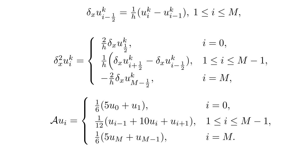
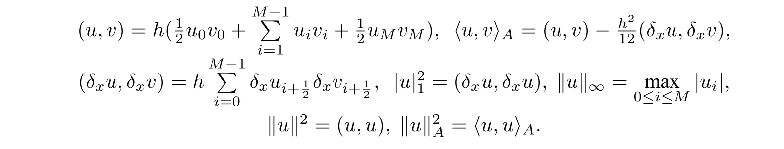
For any grid functionu,v ∈Vh,we further denote

In addition, we denote the fractional differential operatorand the Riemann Liouville fractional derivative,respectively,i.e.,

whereµ=ταΓ(2−α)andbj=(1+j)1−α −j1−α,and

In order to develop a second order approximation to the Riemann Liouville fractional derivative,we introduce the shifted operator defined by

whereωk= (−1)k,k ≥0. We now turn to discretize the Caputo fractional derivative by theL1 formula and the Riemann Liouville fractional derivative.

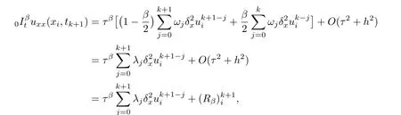
Lemma 2.1([28]) The Caputo fractional derivativeu(x,tk) attk(1≤ k ≤ N) can be estimated by

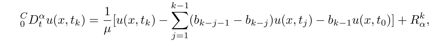
and the truncation errorsatisfies

where the constantcdoes not depend onτ.

Lemma 2.2([12]) Letf(t),−∞Iβ t f(t) and (iω)2−βF[f](ω) belong toL1(R). Define the weighted and shifted difference operator by

then we have

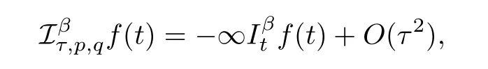
fort ∈R,wherepandqare integers andp ̸=q,andFis the fourier transform of the Riemann Liouville fractional integral.

Lemma 2.3([12]) If(p,q)=(0,−1)in Lemma 2.2,then we have

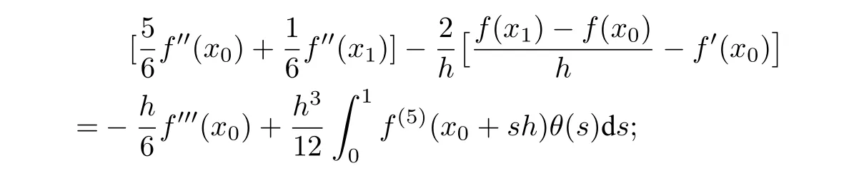
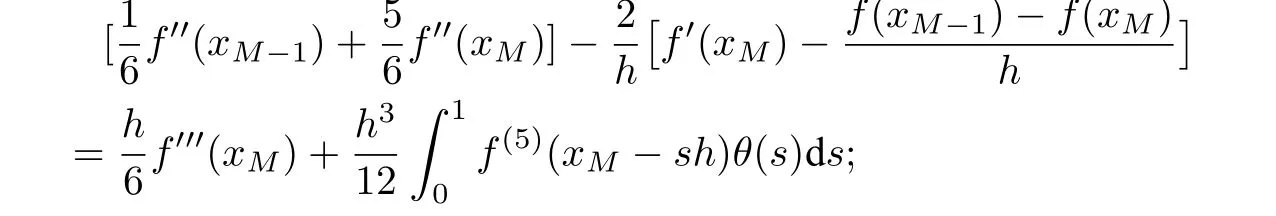
Lemma 2.4([28]) Letθ(s)=(1−s)2[1−(1−s)2]andξ(s)=(1−s)3[5−3(1−s)2].(i)Iff(x)∈C5[x0,x1],then

(ii)Iff(x)∈C5[xM−1,xM],then

(iii)Iff(x)∈C6[xi−1,xi+1],1≤i ≤M −1,then

Inspired by[23]and [28], we next construct the compact difference scheme for solving Eq. (1.1)–(1.3).

Consider Eq.(1.1)at the point(xi,tk),we have

Acting the compact operatorAon both sides of the above equation,it leads to

Fori=0,by Lemma 2.1,Lemma 2.3 and Lemma 2.4(i),we have

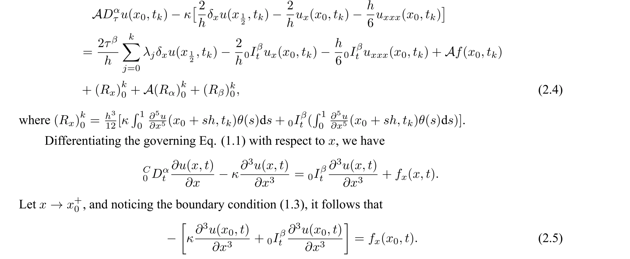
Substituting(2.5)into(2.4)and noticing the boundary condition again,we obtain

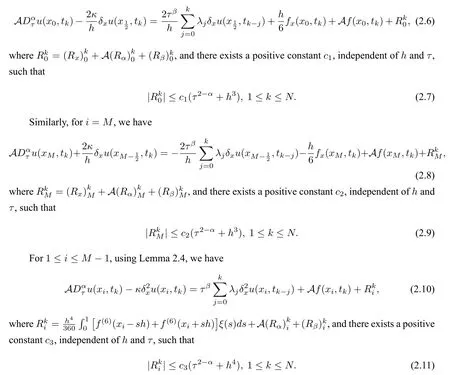
Omitting small termsin(2.6),(2.8)and(2.10),replacing the functionu(xi,tk)with its numerical approximation,we can construct the following compact finite difference scheme

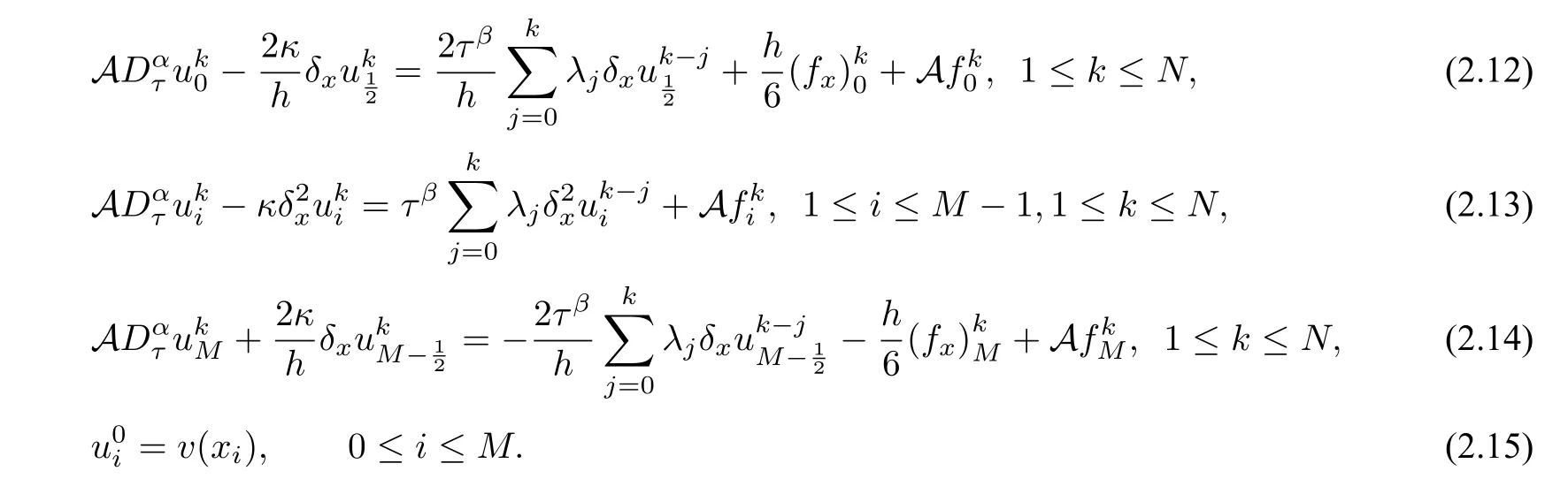
It is easy to see that at each time level, the difference scheme (2.12)–(2.15) is a linear tridiagonal system with strictly diagonally dominant coefficient matrix, thus the difference scheme has a unique solution.

3 Stability and convergence

In this section,we study the stability and convergence of the above compact finite difference scheme.To begin with,we introduce some lemmas,which will play important roles in later analysis.

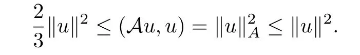
Lemma 3.1([31]) For any mesh functionu ∈Vh,it satisfies

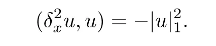
Lemma 3.2([30]) For any mesh functionu ∈Vh,it satisfies

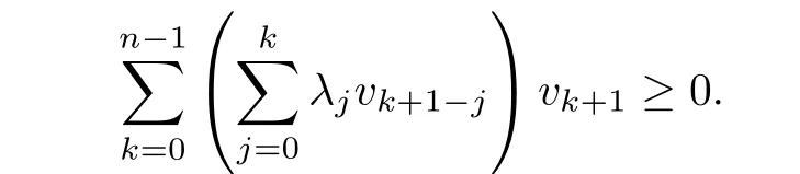
Lemma 3.3([12]) Let{λj}be defined as in Lemma 2.3,then for any positive integerkand real vector(v1,v2,...,vk)T ∈R,it holds that

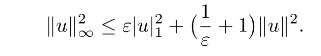
Lemma 3.4([29]) For any mesh functionu ∈Vhand any positive constantε,it holds:

Lemma 3.5([4]) The coefficientsbkin Lemma 2.4,k=0,1,... N,0<α<1,satisfy:

We now turn to prove the stability of the scheme.

Theorem 3.1Let{|0≤i ≤M,0≤k ≤N}be the solution of the following difference scheme,

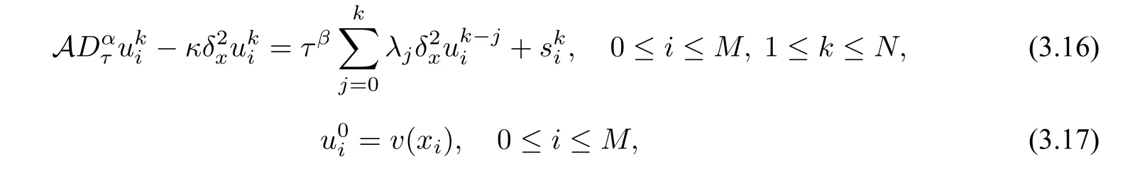
then it holds that

ProofTaking the inner product of(3.16)withµuk,then we have

Summing the above equation(3.19)fromk=1 toN,we get

For the first term on the left,by Lemma 3.1 and the inequalityab ≤,we obtain

Notice that

and

Inserting(3.22)and(3.23)into(3.21),we arrive

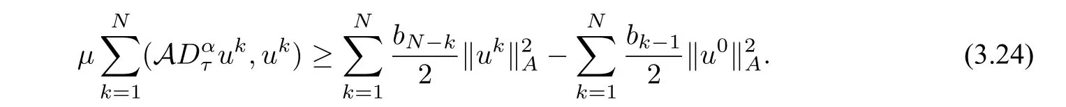
By Lemma 3.2,we get

and by Lemma 3.3 and the inequalityab ≤,we have

Substituting(3.24)–(3.26)into(3.20),and multiplying the result byτ1−α,we deduce

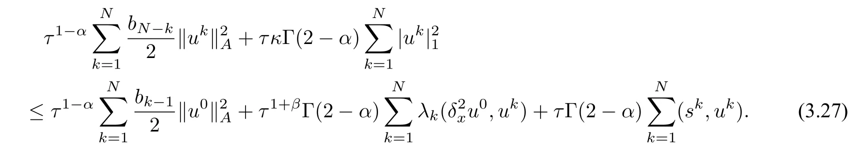
and

Using the Cauthy Schwarz inequality and the result of Lemma 3.4 withε=1,we get

Then we can easily get

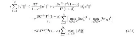
The proof is completed.

Next,we consider the convergence of our scheme. Let

Theorem 3.2Assume thatu(x,t)∈[0,1]×(0,T]is the solution of(1.1)and{uki|0≤i ≤M,0≤k ≤N}is a solution of the finite difference scheme(2.12)–(2.15). Then there exists a positive constant ˜cwhich does not depend onτandhsuch that

ProofWe can easily get the following error equation

Utilizing(2.7),(2.9)and(2.11),it follows from Theorem 3.1 that

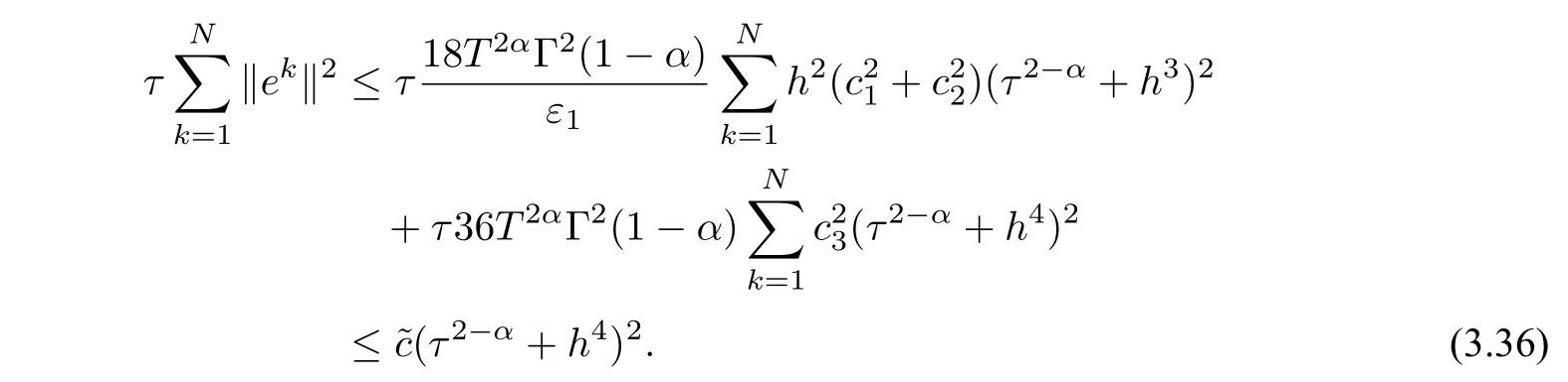
The proof is completed.

4 Numerical experiments

In this section,we carry out some numerical experiments for our compact finite difference scheme.We supposeT=κ=1. The maximum norm errors between the exact and the numerical solutions is

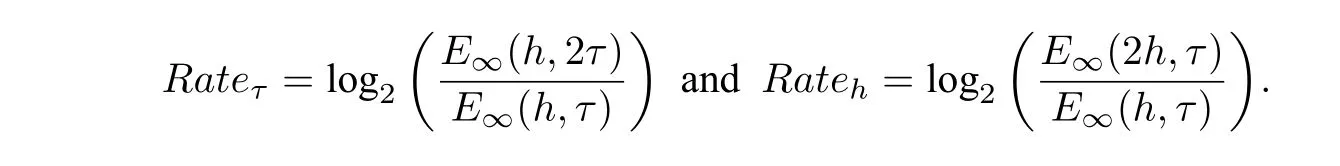
The temporal convergence order and spatial convergence order are respectively

Example 4.1 Suppose

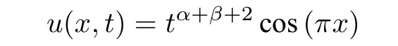
be the exact solution for(1.1),so the associated forcing term is

We firstly investigate the temporal errors and convergence order of the compact difference scheme.Whenβ= 0.3 is fixed, we choose differentα(α= 0.1,0.6,0.9)to obtain the results listed in Table 1,which gives the convergence rate close to 2−α.

Then we test the spatial error and convergence orders. Let the temporal stepτ=is fixed to eliminate impaction of temporal errors. We chooseα= 0.3 andβ= 0.5 in Table 2 to present the maximum errors and the corresponding convergence orders. The numerical results show the spatial fourth order convergence rate. The convergence order of the numerical results matches that of the theoretical one.

Table 1 Numerical convergence orders in temporal direction with h= for Example 4.1

Table 1 Numerical convergence orders in temporal direction with h= for Example 4.1

τ α=0.1 α=0.6 α=0.9 E∞(τ,h) Rateτ E∞(τ,h) Rateτ E∞(τ,h) Rateτ 1/40 3.1295e 5 ∗ 2.4942e 4 ∗ 1.8678e 3 ∗1/80 7.6473e 6 2.0329 1.0309e 4 1.2747 8.9138e 4 1.0672 1/160 1.8620e 6 2.0381 4.1211e 5 1.3228 4.2084e 4 1.0828 1/320 4.5181e 7 2.0431 1.6153e 5 1.3512 1.9757e 4 1.0909 1/640 1.0924e 7 2.0482 6.2549e 6 1.3687 9.2482e 5 1.0952

Table 2 Numerical convergence orders in spatial direction with τ = when α = 0.3, β = 0.5 for Example 4.1

Table 2 Numerical convergence orders in spatial direction with τ = when α = 0.3, β = 0.5 for Example 4.1

h E∞(h,τ) Rateh 1/4 1.0523e 3 ∗1/8 6.4570e 5 4.0266 1/16 4.0174e 6 4.0065 1/32 2.5104e 7 4.0003 1/64 1.5925e 8 3.9786

5 Conclusion

In this paper, the numerical solution for a fractional integro differential equation with Neumann boundary is considered, where the global convergence orderO(τ2−α+h4) is obtained. The difficulty caused by the boundary conditions is handled carefully. The stability and convergence of the finite difference scheme are proved. Numerical experiments are carried out to justify the theoretical result.