CHEN Xi, CHEN Jianqiang, DONG Siwei, XU Guoliang, YUAN Xianxu,*

(1. State Key Laboratory of Aerodynamics, Mianyang 621000, China; 2. Computational Aerodynamics Institute of China Aerodynamics Research and Development Center, Mianyang 621000, China)

Abstract：The stability of leeward streamwise vortices over a Mach 6 yawed cone with 6 degree angle of attack is investigated by using direct numerical simulation (DNS) and stability analyses including spatial BiGlobal and plane-marching parabolized stability equations (PSE3D). It is found that a pair of strong streamwise vortices inducing low-speed mushroom structure simultaneously emerge in the vicinity of the leeward plane. Theoretical results indicate that both low-frequency sinuous modes and high-frequency varicose modes may play an important role in the breakdown of the streamwise vortices.

Keywords：instability of streamwise vortices；hypersonic boundary layer flow； DNS；spatial BiGlobal method；PSE3D method

0 Introduction

Laminar-turbulent boundary layer transition is one of key factors affecting vehicles that operate atsustained hypersonic speeds. A cone at a certain angle of attack (AoA) is frequently encountered in practice, and at the same time is also one of the simplest flow configuration to study the three-dimensional boundary layer transition. For a yawed cone, the pressure within the windward plane is much higher than that within the leeward plane. The resulting pressure gradient drives the fluid to move away from the windward plane towards the leeward plane, inducing strong cross flow in between and a pair of counter-rotating streamwise vortices near the leeward plane. The cross flow may support crossflow instabilities which eventually lead to turbulence through secondary

instabilities, as has been extensively investigated[1-2]. On the other hand, although the transition within the leeward plane has been experimentally measured under various conditions[3-4], numerically documented[5]and theoretically considered[6], the underlying mechanism remains largely unclear.

Since the leeward transition is most likely caused by the breakdown of streamwise vortices, the corresponding transition mechanism may thus be similar to other flow configurations with streamwise vortices being dominant. A typical example is the centerline transition of the HIFiRE-5 elliptic cone at zero AoA. Similar to the yawed cone, spanwise pressure gradients also cause cross flow over the elliptic cone surface and induce a pair of streamwise vortices and a mushroom-like low-speed streak around the center line. Since the centerline flow structures exhibit prominent variations in both the span and wall-normal directions, two-dimensional stability analysis or BiGlobal analysis should be utilized in order to adequately predict the stability characteristics along the center line. Choudhari et al.[7], without accounting for curvature effects, are the first to perform BiGlobal calculations for the centerline stability. Their results highlighted the necessity of considering spanwise variations in the vicinity of the center line. Through spatial BiGlobal analysis with the curvature effects being taken into account, Paredes and Theofilis[8-10]showed the coexistence of varicose and sinuous centerline modes whose wavenumbers and growth rates are nearly coincident at a low unit Reynolds number (1.89 × 106/m). Later, Paredes et al.[11]analyzed a larger unit Reynolds number (1.015 × 107/m) case for the same model, and found that the varicose mode is more unstable. The differences of these two cases are attributed to different mode distributions that the centerline instabilities in the latter case peak closer to the symmetry plane than those in the former, and thus are more sensitive to the symmetry characteristics. Recently, Li et al.[12]demonstrated that varicose and sinuous modes both possess two branches of instabilities, i.e., Y mode and Z mode. Y mode, similar to the unstable modes identified by Paredes and his coworkers, locates at the shoulder region of the mushroom structure, while Z mode resides in the stem region, with lower phase velocities, growth rates and frequencies than Y mode. Choudhari et al.[13]considered the centerline instabilities of the elliptic cone at a small AoA (-1.2°) under the HIFiRE5b flight experiment condition at one instant where a cold wall condition was prescribed. Their PSE3D results showed that sinuous fluctuations can first reach a peak N-factor of approximately 15 at the transition location estimated from the flight data. Similar centerline vortex structures also emerge in another flight model, BoLT. The centerline instabilities were experimentally measured[14-16]and numerically calculated via the dynamic mode decomposition method[17]. Their results indicate the presence of low-frequency disturbances. Nevertheless, detailed instability characteristics remain to be solved through extensive stability analyses. Beside the centerline structures on these three dimensional boundary layers, Görtler vortices in a concave wall also manifest as a pair of counter-rotating streamwise vortices as well as low-speed mushroom structures. In contrast to the centerline instabilities of the elliptic cone, varicose and sinuous modes of Görtler vortices exhibit quite different characteristics concerning with growth rates, frequencies and mode shapes (see, e.g., recent works of Chen et al.[18]and Li et al.[19]).

In this paper, the boundary layer transition in the vicinity of the leeward plane on a yawed cone at Mach 6 is studied with help of DNS and stability analyses for the first time. The objective is to uncover the underlying transition mechanism, and to make comparison with other streamwise-vortices transitions.

1 Flow configuration and basic state

The model (Fig.1(a)) in the present study is a 7°straight circular cone with a nose radius of 1 mm placed at 6°angle of attack. The incoming flow conditions correspond to a free-stream unit Reynolds number of 1.0×107/m, Mach number of 6, static temperature of 79 K. Isothermal wall condition is utilized with the wall temperatureTW=300 K. The direct numerical simulation of boundary layer transition over the whole model was carried out using the OpenCFD developed by Li et al.[20]. The simulation strategy consists of two steps. First, the steady base flow of the entire cone is computed using the finite-volume algorithm with a second-order accurate scheme. In the second step, the calculated steady flow serves as initial and out-boundary conditions for the transition simulation which is performed for a smaller block (X∈[50 mm,700 mm]) without the nose part of cone. In the transition simulation, the inviscid fluxes are computed by using a seventh-order weighted essentially nonoscillatory (WENO) finite-difference scheme, while the viscous fluxes are discretized using a sixth-order central difference scheme. The time integration is performed using a third-order Runge-Kutta scheme. Steady blowing and suction fluctuations (wall-normal velocity varying in the range of ±0.1% of streamwise velocity), randomly distributed in the azimuthal and streamwise direction are forced in the range ofX∈[90 mm, 100 mm] to trigger the transition (see also Li et al.[5]).

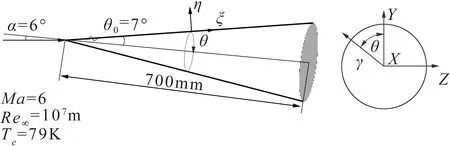
(a) Sketch of the cone model with the body oriented coordinate and flow conditions

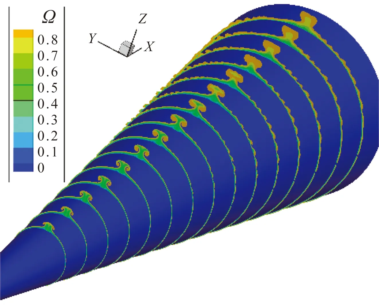
(b) Crossplane contours of streamwise velocity are shown at axial locations from X=120 mm to 350 mm with a step of approximately 16.4 mmFig.1 Model and time-averaged flow structure图1 模型和时均流场结构

A structured grid is used, with 3000 in the axial direction, 1500 in the azimuthal direction, and 300 in the surface normal direction, amounting to a total of 1.35 billion grid points. The grid convergence has been examined by comparing the base flow with a coarse grid with 0.5 billion points and the discrepancy is negligible.

Figure 1(b) depicts the crossplane contours of time averaged streamwise velocity at selected stations along the cone length from the transition simulation. The velocity contours clearly indicate a roll up of low-speed fluid forming a huge mushroom structure in the vicinity of the leeward symmetry plane, along with a series of nearby cross vortices. The pair of vortex structures within the sides of the mushroom cap appear to be lifted up in the downstream due to the self induction of vortices in parallel, resulting in a rapid growth of the height of the mushroom structure.

2 Linear stability theory

2.1 Spatial BiGlobal method

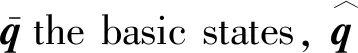
We consider the stability characteristics in the cross-section by decomposing the flow field in a body-oriented coordinate system as follows

(1)

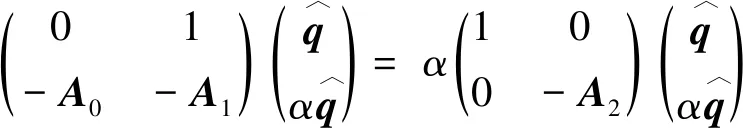
(2)

for the spatial approach whereαis to be solved withωbeing given. Here,A0,A1,A2are linear operators. The boundary conditions are

(3)

These linear operators are discretized using the fourth order finite difference scheme in theηdirection. Since we only focus on the modes whose mode shapes exclusively concentrate within the mushroom structure, the eigenvalue problem is not sensitive to the spanwise boundary conditions so that we can simply apply periodic boundary conditions and use Fourier collocation method in theθdirection. The eigenvalues are then determined by using the Arnoldi’s method. Because of the azimuthal symmetry of the basic state, the disturbances within the mushroom structure can be divided into symmetric (varicose) and antisymmetric (sinuous) modes on the basis of the distribution of the temperature perturbation. The sinuous modes are associated with zero temperature fluctuations at the symmetry plane, whereas the varicose modes have zero azimuthal temperature gradient fluctuations. Therefore, we only need to consider one side of the symmetry plane. The grid distribution and points number have been adjusted to assure the convergence of the eigenvalues.

2.2 PSE3D method

In contrast to the local stability analysis introduced above, PSE3D incorporate initial conditions and nonparallel effects. In the PSE3D formulation, the disturbance is decomposed into a rapidly varying wave-like part and a slowly varying shape function as follows

(4)

(5)

(6)

where

(7)

and the asterisk denotes the complex conjugate. This iteration continued until the latest change was less than 10-5. Note that the curvature effects have been included in the linear operators of both BiGlobal and PSE3D.

3 Results and discussion

3.1 Theoretical results

Figures 2 and 3 show development of growth rates fromX=80 mm throughX=280 mm for unstable varicose and sinuous modes, respectively. It can be observed that leeward-plane instabilities are continually enhanced before approximatelyX=200 mm, and are gradually stabilized further downstream. For the varicose modes, modes V1 and V2 first appear; mode V1 remains to be mild, with the peak frequency increasing from around 50 kHz to 120 kHz in the downstream direction; after a rapid growth between the first two slices, mode V2 becomes dominant except at the fourth slice where mode V4 with higher frequencies is most unstable; other modes possess moderate growth rates, and thus may play a secondary role during the transition process. The results for the sinuous modes closely resemble those for the varicose modes. The most prominent discrepancy is that the low-frequency modes, S1 and S6, appear to be always dominant.

The similarity and difference between the varicose and sinuous modes can be further illustrated by Fig.4 which compares the growth rates and phase velocities, and by Fig.5 which compares the mode shapes atX=200 mm. Several observations can be made. First, each varicose-sinuous mode pair (with the same mode number, e.g. modes V1 and S1) bear a strong resemblance in phase velocities and mode shapes, while the growth rates may differ greatly. Second, the modes can be roughly divided into two groups according to phase velocities and mode shapes. Modes V1, V6, S1 and S6 possess low phase velocities (≈0.8) and reside almost exclusively in the stem region of the mushroom structure. Therefore they are conveniently referred to inner modes. The other modes possess higher phase velocities (≈0.9) and mainly concentrate on the shoulder region, hence can be referred to outer modes. It is interesting to note that the inner modes look similar to the “Z mode” of centerline instability for the HIFiRE-5 elliptic cone[12]and the stem mode of secondary instability for Görtler vortices[18-19,21], while the outer modes appear to be closely related to the “Y mode” of centerline instability for the HIFiRE-5 elliptic cone[10,12]and other modes than the stem mode for Görtler vortices. Since inner modes lie closer to the symmetry plane of the mushroom structure than the outer modes do, inner modes are thus more sensitive to the symmetry than outer modes. This explains why the inner modes exhibit remarkable discrepancies in growth rates for each varicose-sinuous mode pair, while the growth rates of each varicose-sinuous outer modes nearly coincide. Similar phenomenon has also been observed by Choudhari et al.[13]in the HIFiRE-5 model.

(a) Growth rate

Fig.4 Comparison of growth rate and phase velocity of unstable varicose modes (filled symbols) and sinuous modes (unfilled symbols) atX=180 mm

图4X=180 mm站位处，对称模态(实心符号)和 反对称模态(空心符号)的增长率和相速度分布对比

Fig.5 Comparison of normalized mode shapes (temperature) for the unstable varicose modes V1～V6 (a～f) and sinuous modes S1～S6 (g～l) at X=200 mm. The frequency is chosen to be the most unstable component of each mode. The temperature base flow is also displayed.图5 X=200 mm站位处的六个对称模态(a～f)和反对称模态(g～l)的形状函数(温度)分布对比 (所选频率是各个模态最不稳定的分量, 温度基本流用实线表示)

Figure 6 displays the normalized amplitude distribution of the streamwise velocity gradient components, |∂U/∂η| and |∂U/∂θ|. It can be observed that the instabilities all reside in the high-shear regions. In particular, modes V1, V3, V4 and V6 appear to be associated with the spanwise shear, while the other modes seem to be related to the wall-normal shear. The same holds for the sinuous modes.

(a) |∂U/∂η| (b) |∂U/∂θ|

Fig.6 The normalized amplitude distribution of the streamwise velocity gradients atX=200 mm (The solid lines show the streamwise velocity contours)

图6 归一化后的流向速度梯度,X=200 mm (实线表示流向速度等值线)

At last, the spatial structures of the dominant varicose and sinuous modes atX=120 mm andX=200 mm are reconstructed in Fig.7. The relative positions of the outer modes (a, c) and the inner modes (b, d) are clearly shown. In the upstream, the dominant varicose mode resides in the top of the mushroom structures, which is similar to the typical varicose instability of Görtler vortices (see e.g. Chen et al.[18]). At the next slice, both instabilities manifest as helical structures, as are also observed in the HIFiRE-5 model[9], the BoLT model[17,22]and Görtler vortex flows[23].

To characterize the axial evolution of the unstable disturbances and establish a topological connection between the mode shapes at different axial stations, PSE3D are performed across a range of mode frequencies. The amplitude evolutions shown in Fig.8(a) clearly indicate that sinuous modes (solid lines) can reach much higherN-factors than varicose modes (dashed lines) do, of which the most amplified sinuous component is 80 kHz while the most amplified varicose components are 120 kHz originating from V2 and 260 kHz from V4. Figures 8(b, c) compares the amplitude evolutions obtained by DNS, BiGlobal and PSE3D for the most amplified varicose component 260 kHz and sinuous component 80 kHz, respectively. Two observations can be made. First, the theoretical results favorably agree with the DNS results. The discrepancies in the beginning and in the late stage are attributed to the transient behaviors of DNS disturbances (i.e., consisting of multiple types of fluctuations) and nonlinear effects of disturbances (appearing first in the varicose mode), respectively. Second, PSE3D and BiGlobal results are very close except for the initial stage where the initial profiles provided by BiGlobal will undergo a transient stage in PSE3D.

The mode shape evolution of the dominant varicose (260 kHz) and sinuous (80 kHz) modes are shown in

Fig.7 Spatial structures illustrated by isosurfaces of normalized temperature mode shape (±0.2) for mode V2, mode S1 atX=120 mm, and of mode V4 and mode S1 atX=200 mm, together with the base flow isosurface (1.87Te) (The streamwise scale is equal to two wavelengths of each mode)

图7 温度等值面显示的模态空间结构(流向尺度为两个模态流向波长)

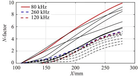
(a) N-factors obtained by PSE3D for some sinuous modes (solid lines) and varicose modes (dashed lines); the most amplified modes have been labelled

(b) The varicose mode of 260 kHz

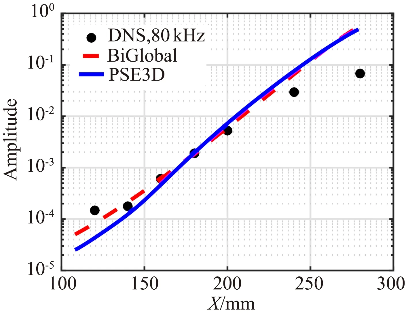
(c) The sinuous mode of 80 kHz

Fig.8 Disturbance amplitude evolution of a single frequency. Comparison of amplitude evolutions from DNS, BiGlobal and PSE3D have been made for two most amplified mode. Note that the amplitude from DNS is obtained by the average of the (fast Fourier transformation) amplitudes in certain frequency bands (250～270 kHz and 70～90 kHz).

图8 PSE3D预测的单频扰动幅值演化(N值曲线)及与BiGlobal和DNS结果的对比(其中N值曲线中不同模态最不稳定的频率分量用彩色线条标记)

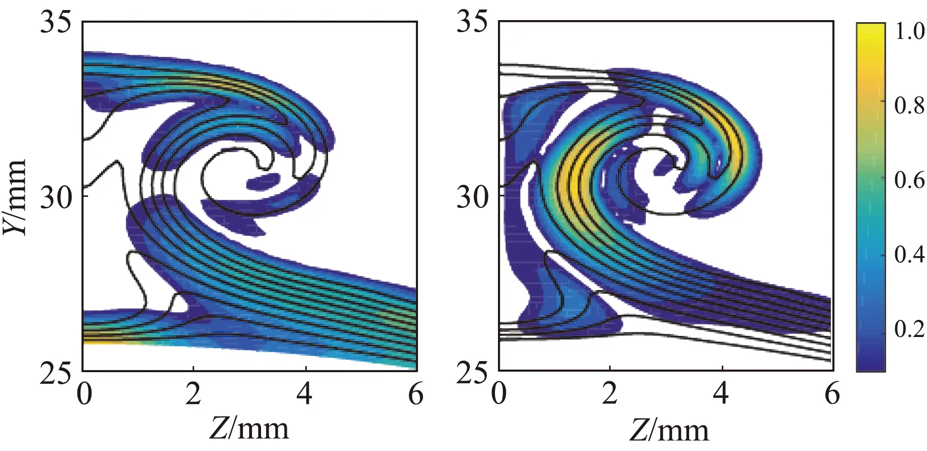
Figs.9(a-f) and (h-l), respectively. For the varicose mode, the disturbances initially locate at the mushroom cap, and gradually shift down to the shoulder region with another small peak emerging in the inner side since the slice of Fig.9(c). In contrast, the fluctuations of the sinuous mode reside in the stem region in the upstream region, and gradually spread outwards along with the rolling of the fluid, inducing another peak in the cap.

3.2 Statistic results from DNS

In this subsection, the statistic results from DNS are presented to highlight the transition process upon comparison with the results from the stability analyses above. Figure 10 displays the normalized r.m.s. distribution at three streamwise slices. The spectra obtained at the local r.m.s. peak positions are also shown. In the upstream, the disturbances concentrate on the top of the mushroom structure, which is consistent with the predominance of mode V2 there (see Fig.7(a)). However, the corresponding spectrum exhibits a peak frequency of approximately 600 kHz, nearly three times higher than the dominant frequency (around 200 kHz) of mode V2. Where such high-frequency disturbances arise is unclear yet. At the next slice, r.m.s. distribution forms new local maximums in the shoulder and stem regions of the mushroom structure, in addition to a weak one on the head. The dominant disturbance frequencies for the head region are in range of [160 kHz, 220 kHz], and move to a slight higher frequency range for the shoulder region. The spectra and the filtered r.m.s. distribution (in Fig.11) indicate that the disturbances at these two regions consist of the outer modes, of which the disturbances at the shoulder region likely evolve mode V4/S4 with the disturbances in the head region being mainly contributed by other outer modes. At the stem region, two peaks appear in the spectrum, one similar to that at the shoulder region, the other one lying in a much lower frequency range, which indicates the coexistence of two types of instabilities there. Comparison between the filtered r.m.s. distribution (Fig.11(c)) with the mode shapes from the PSE3D results indicates that the low-frequency peak corresponds to mode S1. For the last slice, the r.m.s. has spread to the whole mushroom structure. The spectrum at the shoulder region displays a broad plateau for [0,200 kHz], while the spectrum at the stem region shows a prominent peak at approximately 90 kHz. The high-frequency disturbances in the range of [200 kHz, 400 kHz] become relatively insignificant compared to the spectra at the previous one. This trend is consistent with the results of stability analyses which predict that low-frequency instabilities gradually take over in the downstream region.

Fig.9 Mode shape (normalized temperature fluctuations) evolution of the dominant varicose mode at f=260 kHz (a～f) and of the dominant sinuous mode at f=80 kHz (g～l) predicted by PSE3D. The slices start from X=112.7 mm to X=261.7 mm with a step of approximately 28 mm. The temperature base flow is shown by the solid lines.图9 PSE3D得到的最不稳定对称模态(260 kHz)和反对称模态(80 kHz)的形状函数沿流向的演化

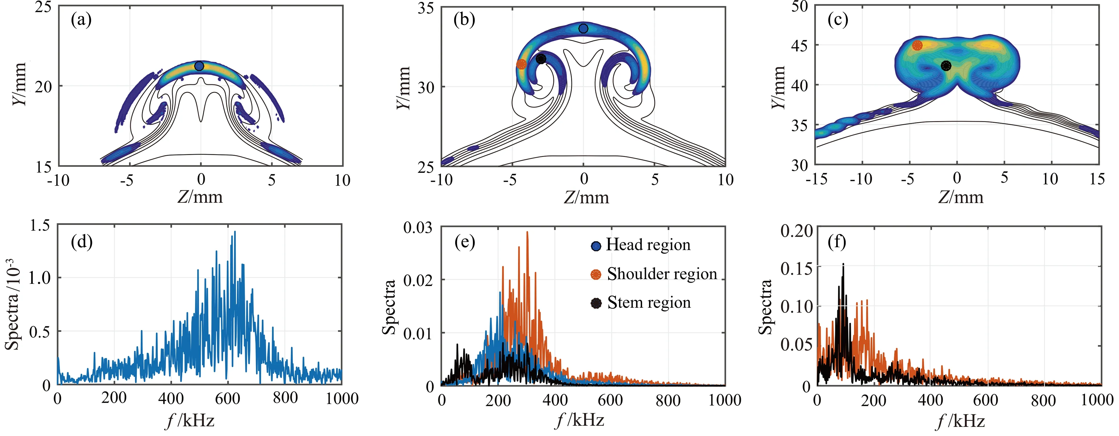
Fig.10 Normalized root-mean-square distribution of temperature disturbances at three slices, (a)X=120 mm, (b)X=200 mm, (c)X=280 mm, together with the base flow isolines. The corresponding spectra at the sampling points (denoted by the symbols) are also shown in (d,e,f).

图10 三个流向站位处的DNS扰动均方根分布和极值点处的频谱

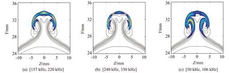
Fig.11 Normalized root-mean-square distribution of temperature disturbances over certain frequency ranges at X=200 mm, together with the base flow isolines.图11 X=200 mm处DNS特定频段处的扰动均方根分布

4 Conclusions

In this paper, sophisticated stability analyses (spatial BiGlobal and PSE3D) and DNS are performed to reveal the leeward-plane transition mechanisms on a hypersonic yawed cone for the first time. The low-speed mushroom structure induced by the leeward streamwise vortices is shown to be susceptible to multiple unstable modes. The unstable modes can be further classified as outer modes and inner modes. Outer modes with higher phase velocities and frequencies, reside in the shoulder and head regions of the mushroom structure, whereas inner modes being located at the stem region possess lower phase velocities and frequencies. Both outer modes and inner modes contain varicose and sinuous components. The sinuous components dominate for inner modes, while for outer modes the varicose components are more unstable in the upstream but gradually collapse with the sinuous components in the downstream. Good agreement between the stability analysis and DNS results are obtained, except that the disturbances from DNS in the upstream region show much higher frequencies than prediction.

Stability of leeward streamwise vortices is found to bear a remarkable resemblance with instabilities of streamwise vortices in other flow configurations (e.g. elliptic cone, the BoLT model and Görtler vortex flows) in the sense that varicose and sinuous instabilities coexist, covering a wide unstable frequency range from tens to hundreds of kHz.