Fei Qingyi Kong Nan Zhao Lindu

(1School of Economics and Management, Southeast University, Nanjing 211189, China)(2Weldon School of Biomedical Engineering, Purdue University, West Lafayette IN 47907, USA)

Abstract：To balance inventory cost with diverse demand, an optimal investment decision on necessary process improvement for delayed product differentiation is studied. A two-stage flexible manufacturing system is modeled as a continuous time Markov chain. The first production stage manufactures semi-finished products based on a make-to-stock policy. The second production stage customizes semi-finished products from the first production stage on a make-to-order policy. Various performance measures for this flexible manufacturing system are evaluated by using matrix geometric methods. An optimization model to determine the level of investment on process improvement that minimizes the manufacturer’s total cost is established. The results show that, a higher investment level can reduce both the expected customer order fulfillment delay and the expected semi-finished products inventory. When the initial order penetration point is 0.4, the manufacturer’s total cost is reduced by 15.89% through process investment. In addition, the optimal investment level increases with the increase in the unit time cost of customer order fulfillment delay, and decreases with the increase in the product value and the initial order penetration point.

Key words：flexible manufacturing system; postponement strategy; order penetration point; investment process; matrix geometric method

In the era of e-commerce and make-to-order (MTO) manufacturing, customer purchase behavior has a pronounced impact on the manufacturer’s production process. Many customers prefer more personalized products that satisfy their specific needs, while others are unwilling to wait long for customized products and prefer standard products on a guaranteed order delivery time. Such diverse customer purchase behaviors require the production process to be flexible while ensuring its productivity[1]. Consequently, the postponement strategy is adopted to match the various behaviors.

The postponement production system is usually composed of two phases, namely, push and pull. On the one hand, the push phase is forecast-driven. It is located upstream and follows standard production. On the other hand, the pull phase is customer-driven. It is located downstream and follows customized production. The order penetration point (OPP) is the boundary between these two phases, which is also known as the point of differentiation or the customer order decoupling point. Given the importance of the postponement strategy, the OPP decision problem has attracted much attention in the literature.

There are two main lines of literature related to our study, i.e., OPP decision-making with and without consideration of any process improvement. We first review the literature without considering any process improvement. Jewkes et al.[5]found that the optimal OPP moves downstream if customers accept a narrower range of product characteristics. However, the optimal OPP is neither sensitive to the changes in supplier capacity nor customer demand. Pang et al.[6]proposed a cost control model with multiple product differentiation points, and analyzed the implementation conditions of process flow reorder. Zhang et al.[7]presented a supply chain postponement strategy model by using the queuing theory to determine the optimal ratio of differentiation and inventory level. Shao et al.[8]modeled various postponement strategies for coping with risk in the thin film transistor liquid crystal display industry. Shan et al.[9]investigated the application of the postponement strategy in apparel supply chain management. They found that it is beneficial to adjust the first production proportion and replenishment ratio to improve competitiveness. Liu et al.[10]proposed an OPP decision model considering time scheduling with capacity and time constraints. Numerical examples showed that OPP moves earlier with the increase in the volume of new orders. Yousself et al.[11]studied the impact of items priority levels on the optimal MTO/MTS decisions. By setting the optimal priority allocation and the base-stock levels, the overall inventory costs are minimized. Nevertheless, the studies discussed above only explored the relationship between the optimal OPP and the postponement strategy. Little investigation has been done on the relationship between OPP and the investment process.

The literature on the impact of process improvement on the OPP decision-making is still in its infancy. Lee[12]was the first to present inventory models for product/process design applications. Those models, however, assume that no buffer stocks are held until the end of the production process. In a further developed model, Lee et al.[2]allowed different process points to hold inventories and incorporated several factors that would normally be affected by delayed product differentiation. However, the average investment cost per period is independent of OPP in their model. Su et al.[13]considered the problem that a firm can make a series of investments to design generic product components with the implementation of postponement structure. However, the one-time investment cost is assumed to be fixed in their model. More recently, Ngniatedema et al.[14]extended the model[2]by incorporating the delivery of product components from an external supplier at the beginning of the production network. However, the investment cost remains independent of OPP.

In our paper,OPP can be pushed downstream through process investment. We model the production process to better understand how the investment level affects the trade-off between customer order fulfillment delay and inventory risks. We use an approach similar to that proposed by Jewkes et al.[5]and propose an alternative model. First, our model is used to investigate the impact of the investment level on the postponement strategy instead of market characteristics[5]. Secondly, the investment level is regarded as a decision variable in our model, not a fixed value. In addition, we assume that the updated OPP through process improvement meets the law of diminishing marginal utility, and thus it is modeled with a continuous, increasing, and concave function with respect to the investment level.

1 Production System Model

For each type of product that the manufacturer offers, the production system consists of two phases. In phase one, the semi-finished parts are made in an MTS fashion, and are stocked at the warehouse. In phase two, when the manufacturer receives customer orders, the semi-finished parts are customized in an MTO fashion and are sent directly to customers. Fig.1 illustrates the postponement production process.

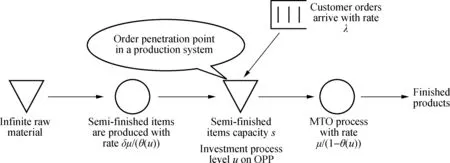
Fig.1 The postponement production process

As shown in Fig.1, we assume that the manufacturer can procure an infinite amount of raw materials and never faces shortages. Meanwhile, we assume that it has limited storage capacity for semi-finished products, denoted bys. We quantify the OPP variable, denoted byθ(0<θ<1), to be the percentage of product completion after phase one. We setθ0to be the initial OPP. Note that we useθ, a continuous variable, to quantify the decision about product differentiation, thus it is more convenient to derive analytical results from our model and conduct sensitivity analyses. While most of the production processes are not continuous with respect to OPP, the optimal value obtained from our model can be used in practice to guide the postponement of product differentiation.

1.1 Markov model

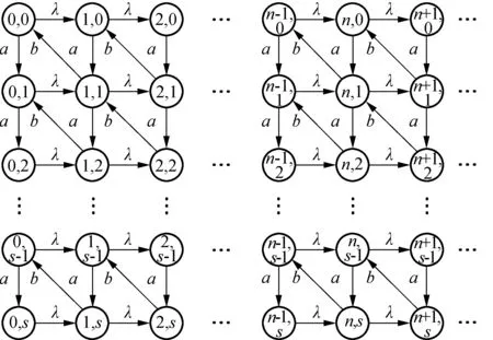
Fig.2 Transition rate diagram of the Markov chain

Letπ={π0,π1,…,πn} be the steady-state probability of the Markov chain, whereπn={π(n,0),π(n,1),…,π(n,s)} is an (s+1)-dimensional row vector. Additionally,π(i,j)denotes the steady-state probability associated with the condition that there areiorders andjsemi-finished products. Referring to the transition diagram in Fig.2, we obtain the following balance equations:

(a+λ)π(i,j)=bπ(i+1,j+1)i=0,j=0

(1)

(a+λ)π(i,j)=aπ(i,j-1)+bπ(i+1,j+1)i=0,1≤j≤s-1

(2)

λπ(i,j)=aπ(i,j-1)i=0,j=s

(3)

(a+λ)π(i,j)=λπ(i-1,j)+bπ(i+1,j+1)1≤i,j=0

(4)

(a+λ+b)π(i,j)=aπ(i,j-1)+λπ(i-1,j)+bπ(i+1,j+1)
1≤i,1≤j≤s-1

(5)

(λ+b)π(i,j)=aπ(i,j-1)+λπ(i-1,j)1≤i,j=s

(6)

The generator matrix of the Markov chain is given by

(7)

where

1.2 Performance evaluation

With the steady-state distribution, we can compute the following queuing performance measures:E(L) is the expected number of customer orders;E(W) is the expected customer order fulfillment delay (i.e., the expected time from customer order arrival to order completion), andE(O) is the expected number of semi-finished products. The measures are then given by

E(L)=π1(I-R)-2D

E(W)=E(L)/λ

E(O)=π0(I-R)-1V,V={0,1,2,…,s}T

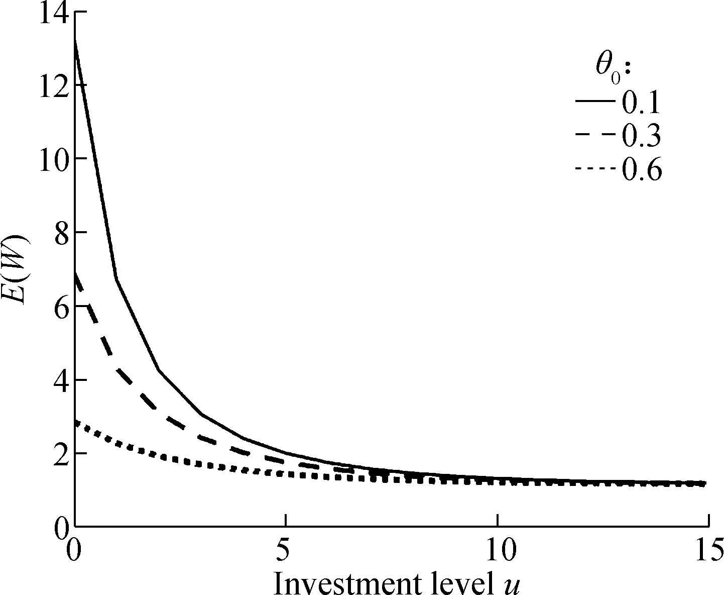
From Fig.4, we observe that a higher investment level results in a shorter expected customer order fulfillment delay. This observation implies that a smaller percentage of the production process is required to perform the customization task, which reduces the expected customer order fulfillment delay. Additionally,E(W) is sensitive toθ0. If the initial OPP is located at the front-end of the production process, the expected fulfillment delay registers a more marked reduction. However, when the process improvement is beyond a certain investment level, such asu=10 in Fig.4(a), the expected customer order fulfillment delay remains unchanged, no matter where the initial OPP is located.

Fig.5 shows howE(O) is affected byu. A higher investment level is beneficial to hold a fewer expected number of semi-finished products. As the investment level increases, the initial OPP is pushed down; i.e., a larger

(a)

(a)

(a)

percentage of each product is completed in advance in phase one. Customers can receive their products much faster. As a result, it is not necessary to hold a more semi-finished products inventory. Similarly to Fig.4,E(O) is also sensitive toθ0. The smaller theθ0, the larger theE(O).

2 Cost-Minimization Formulation

The manufacturer seeks to minimize the sum of the following costs when determining the optimal investment levelu*: The expected cost of customer order fulfillment delay; the expected inventory holding cost of semi-finished products; and process improvement cost. Mathematically speaking, the manufacturer intends to minimize its total cost (TC).

minTC(u)=CwE(W)+ChV(θ)E(O)+gu2

(8)

whereCwis the average cost per time unit of customer order fulfillment delay;Chis the average holding cost per time unit per semi-finished product;V(θ) is the average value per semi-finished product, assumed to be increasing inθ; andgis the cost coefficient of the investment. Here we assume that the cost directly associated with the investment level is quadratically proportional to the investment level. The customer order fulfillment delay may decrease as the investment level increases. However, an increased investment may also increase the inventory holding cost of semi-finished products and also increase spending on the investment. Hence, the manufacturer must weigh these conflicting factors when selecting the optimal investment level.

2.1 Optimization results

Fig.6 shows the manufacturer’s total cost and the OPP under different investment levels whenθ0=0.1. It is noted that the minimum total cost is 7.361 and it occurs when the investment level is 3, i.e.,u*=3. The manufacturer’s total cost is reduced by 48.29% through process investment, which is remarkable. The corresponding optimal OPPθ(u*) is 0.575. Increasing the investment level can indeed lower the manufacturer’s total cost. However, when the investment level further increases, it no longer results in any cost reduction.

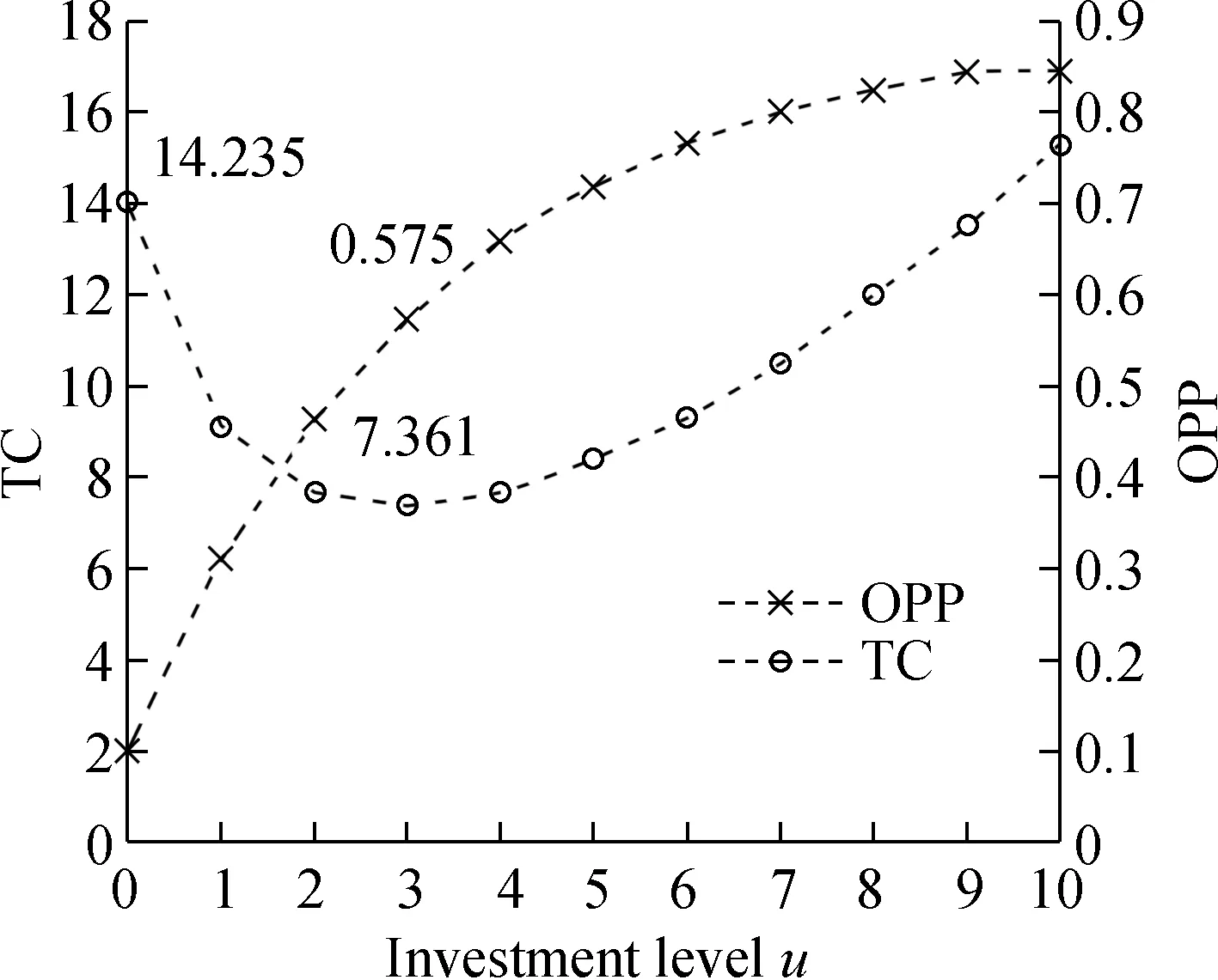
Fig.6 Impact of investment level on total cost and OPP

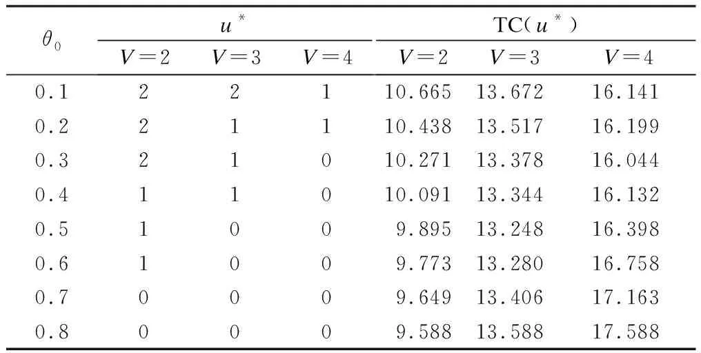
Tab.1 shows the optimal investment levelu*and the optimal OPPθ(u*) with respect to variedθ0. Asθ0increases,u*decreases and is greater than 0. Thus, it is beneficial to further delay product differentiation through process investment, since reducing the customer order fulfillment delay is the primary goal of the manufacturer. However, whenθ0=0.8,u*is reduced to 0. It means that there is no investment. The manufacturer’s total cost increases in response to any further increase in investment, and thus the manufacturer is unwilling to further invest in the process improvement. On the other hand, the optimal OPPθ(u*) does not strictly increase withθ0.θ(u*) declines from 0.615 to 0.571 whenθ0increases from 0.2 to 0.3. The reason is thatu*decreases from 3 to 2. For a similar reason,θ(u*) falls slightly whenθ0increases from 0.5 to 0.6. Fig.7 describes the relationship amongθ(u*),u*andθ0.

Tab.1 The optimal decisions for various θ0

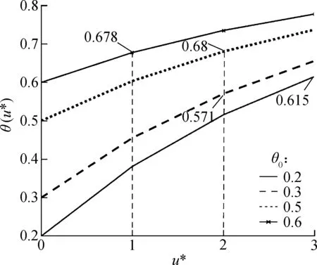
Fig.7 The optimal OPP and optimal investment level under different θ0

2.2 Sensitivity study

Next, we study the sensitivity of optimal solutions with the parameters changing.

Fig.8(a) and Fig.9(a) illustrate that as the unit-time cost of customer order fulfillment delay increases, the optimal investment level and the cost saving rate increase. This implies that, for a higher unit-time cost of customer order fulfillment delay, the manufacturer should more sensibly consider an investment in the process improvement. In other words, the OPP is likely to be further pushed downstream with impatient customers.

As the product value increases in Fig.8(b) and Fig.9(b), the optimal investment level and the cost saving rate decrease. This implies that the manufacturer is less willing to make an investment on process improvement when the product value becomes larger. This is due to an increase in the holding cost of the semi-finished products.

Additionally,as shown in Fig.8(c) and Fig.9(c), the optimal investment level and the cost saving rate decrease with the increase in the cost coefficient of the investment. A higher cost coefficient of the investment means that the manufacturer should invest more in order to achieve the same delivery lead time. To balance the customer order fulfillment delay cost with the investment cost, the manufacturer may set a reasonable investment level.

For more sensitive information, please see Tabs.2 to 4.

(a) (b) (c)Fig.8 Impact of Cw, V, g, θ0 on optimal investment level. (a) V=1, g=0.1; (b) Cw=1,g=0.1; (c) Cw=1,V=1

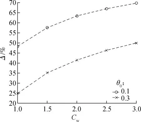
(a) (b) (c)Fig.9 Impact of Cw, V, g, θ0 on cost saving rate. (a) V=1, g=0.1; (b) Cw=1,g=0.1; (c) Cw=1,V=1

θ0u*Cw=1.5Cw=2Cw=2.5TC(u*)Cw=1.5Cw=2Cw=2.50.14448.85110.05211.2540.23448.5099.73310.8340.33348.1749.38610.4490.43347.8808.95710.0970.52337.4938.5779.5340.62227.1338.0959.0570.71226.7377.6478.4640.81116.3587.0917.825

Tab.3 The optimal u* and TC(u*) for various V

Tab.4 The optimal u* and TC(u*) for various g

3 Conclusion

This paper mainly investigates the investment decision optimization for delayed product differentiation. A flexible manufacturing system modeled as a continuous time Markov chain is considered. Two important queuing performance measures by using the matrix geometric method are computed. Furthermore, our study leads to three managerial recommendations. First, the manager should consider the initial OPP when making a decision to invest or disinvest in the process improvement. Secondly, the manager should focus more on impatient customers as the cost of customer order fulfillment delay can have different impacts on the investment decision. Finally, the manager should take a more holistic viewpoint by considering the value of the products and the cost directly associated with the investment decision, especially when attempting to launch a high volume of investment.