Huang Bonan Xia Weiwei Zhang Yueyue Zhang Jing Zou Qian Yan Feng Shen Lianfeng

(National Mobile Communications Research Laboratory, Southeast University, Nanjing 210096, China)

Abstract：In order to solve the problem of efficiently assigning tasks in an ad-hoc mobile cloud (AMC), a task assignment algorithm based on the heuristic algorithm is proposed. The proposed task assignment algorithm based on particle swarm optimization and simulated annealing (PSO-SA) transforms the dependencies between tasks into a directed acyclic graph (DAG) model. The number in each node represents the computation workload of each task and the number on each edge represents the workload produced by the transmission. In order to simulate the environment of task assignment in AMC, mathematical models are developed to describe the dependencies between tasks and the costs of each task are defined. PSO-SA is used to make the decision for task assignment and for minimizing the cost of all devices, which includes the energy consumption and time delay of all devices. PSO-SA also takes the advantage of both particle swarm optimization and simulated annealing by selecting an optimal solution with a certain probability to avoid falling into local optimal solution and to guarantee the convergence speed. The simulation results show that compared with other existing algorithms, the PSO-SA has a smaller cost and the result of PSO-SA can be very close to the optimal solution.

Key words：ad-hoc mobile cloud; task assignment algorithm; directed acyclic graph; particle swarm optimization; simulated annealing

Mobile devices (MDs) have gained enormous popularity in our daily life. As a result, mobile applications running on the mobile devices require much more time and energy. In spite of the significant development in the capabilities of these MDs, compared with computer systems, MDs are still limited by storage, lifetime, and computing abilities, etc. Mobile cloud computing (MCC)[1], by enabling offloading part of the workload to a remote cloud, cloudlet or other MDs, opens up a new possibility to further enhance the MDs computing ability and to extend their storage and lifetime.

The ad-hoc mobile cloud (AMC) consists of a number of nodes with different performances, and each node has the capability to serve both as a server and, at the same time, a client. These nodes communicate over radio and operate without the benefit of any infrastructure, thereby creating an opportunistic resource sharing platform. Such characteristics make AMC an ideal solution for scenarios with weak or no internet connection.

AMC coordinates with MDs which are close to each other to process an application together, and offers an efficient solution for reducing the latency of the MDs applications[2]. Moreover, due to the rapid development of energy harvesting technology, MDs are expected to harvest energy from an ambient environment so as to facilitate self-sustainability and perpetual operation. With energy harvesting capability, MDs are more likely to perform task sharing to maximize the overall utility of the whole network.

Workflow can effectively describe the complex constraint relationships between activities. The directed acyclic graph (DAG) is a common way of describing it. In recent years, the research of DAG scheduling has made great progress. Gotoda et al.[3-4]first proposed the scheduling problem of multi-DAGs sharing a set of a distributed resource. Then, they put forward some solutions to the problems such as the minimization of the make span and the fairness of scheduling. Xu et al.[5-7]also made some improvements on this basis. However, only a few studies have been made on the DAG scheduling with a constraint. In this paper, a DAG model representing the dependencies between tasks under the constraint of time delay is proposed.

Task assignment is also an important part of cloud computing. Many intelligent optimization algorithms such as the genetic algorithm, particle swarm algorithm, ant colony optimization are introduced into the research of the task assignment. In Ref.[8], an improved particle swarm optimization (PSO) algorithm applied to workflow scheduling is studied. Rahman et al.[9]proposed the improved PSO algorithm to make the plan for virtual machine migration. In Ref.[10], the genetic algorithm (GA) is used to optimize the path length and the number of common hops jointly. In Ref.[10], the GA is used to maximize the throughput of the network. Although Truonghuu et al.[11-14]optimized the task assignment in cloud computing in different ways, neither the fairness of the resources’ use nor the interference of the transmission in the wireless network is considered. To fill this gap, this paper proposes a model of wireless network ad-hoc mobile cloud communication, and the total energy consumption of all devices and fairness of resource usage of all devices are considered simultaneously.

The PSO outperforms other population-based optimization algorithms, such as the GA and other evolutionary algorithms, due to its simplicity[15-17]. The efficiency of solving various optimization problems was proved in Refs.[18-21].However, the PSO has disadvantages. It is easy to fall into local optimal solutions, and it shows slow convergence in evolution and poor precision. The SA algorithm has the ability to make it possible to jump out of the trap of local optimal solutions and its convergence has been proved theoretically[22]. The algorithm in this paper combines the particle swarm optimization and simulated annealing with a strong ability to jump out of local optimal solutions, so as to improve convergence speed and precision.

Our main contributions can be summarized as follows:The energy consumption and time delay are regarded as costs at the same time. The dependencies between tasks are converted into a DAG model. The task assignment in the AMC is transformed into an optimization problem and a PSO-SA based algorithm is proposed to solve this complex optimization problem.

1 System Model

The considered ad-hoc mobile cloud is illustrated in Fig.1.Ad-hoc mobile cloud consists of a set of mobile devices connected by a set of wireless links. The device

Fig.1 Task assignment in ad-hoc mobile cloud

which asks for help from neighbors is denoted as a master; in contrast, the device which provides cooperation to the master for offloading is denoted as slave. As shown in Fig.1, Master 0 is connected to each slave via a wireless link and it has a computing-intensive taskQtotalto be calculated, but it does not have enough computing resources to execute them, so Master 0 splitQtotalton+1 parts (Q0,Q1,Q2, …,Qn). Each part is transmitted to a specific slave to be processed or be calculated by local computing. As can be seen from Fig.1,Q0represents the part of tasks calculated by local computing and other parts of tasks are offloaded to different slaves to be calculated. Each task is not independent during the execution, so it is necessary that the slave nodes are also able to collaborate with each other.

1.1 DAG model

LetMrepresent the total number of the tasks. The dependencies of the tasks can be represented by the DAG models. In this paper, a four-tupleG={T,E,W,C} is used to represent the DAG model.

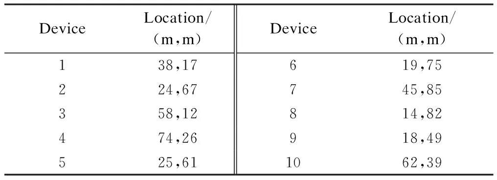
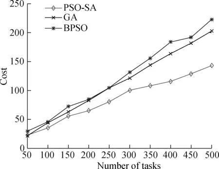
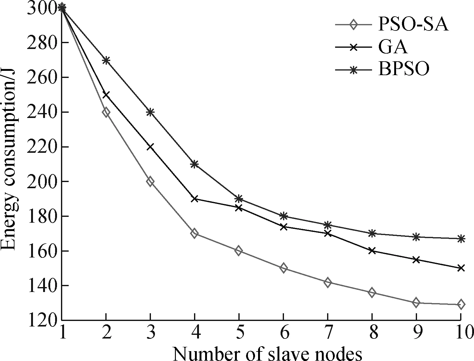
T={eij} is the collection of tasks in the DAG.tirepresents taski, where 0≤i

E={ei,j} is the collection of directed edges,where 0≤i

W={w(i)} is the collection of the computing workload (i.e., the total number of CPU cycles).w(i) denotes taski’s computing workload, where 0≤i≤M.

C={ci,j} is the collection of the size of computation input data (e.g., the program codes and input parameters).ci,jis the size of computation input data from taskito taskj, where 0≤i

In order to give a clearer description of the mathematical model, the following definitions are given：

pre(ti) represents the collection of previous tasks of taski.

suc(ti) represents the collection of succeeding tasks of taski.

tin={t|pre(t)=∅} represents the entry task.

tout={t|suc(t)=∅} represents the exit task.

LetNrepresent the total number of the slave nodes,am∈[1,N] denote the offloading decision of taskm.am=nmeans that taskmis offloaded to slaven. Furthermore, the decision profile is denoted asA=(a1,a2,…,am).

For a given decision profile, the DAG modelGcan be further processed. If two tasks on one edge are assigned to the same node, thenci,jon this edge will be set to be zero, which means that communication energy consumption will not be generated.

Fig.2 shows the dependencies between eight tasks.Let each circle in the figure represent a task;P1,P2,P3andP4represent four nodes; the edge between taskiand taskjrepresents the dependencies between tasksei,j; and the number above the edge between taskiand taskjrepresents the size of computation input dataci,j. For example, as shown in the figure,e2,5=1 ande3,5=1, which means that task 5 relies on tasks 2 and 3.These two tasks are assigned to the same node, so the energy consumption generated by transferring input data can be ignored, which means thatc2,5=0.

Fig.2 The dependencies between tasks

1.2 Communication model and calculation model

According to the decision profileA, the number of the slave nodenwhich taskmis assigned to can be obtained. Then, the slave nodenwill execute the computation taskmand return the results to the master. The execution of taskmin the cloud includes three phases: The transmitting phase, the computing phase, and the receiving phase.

In this paper, the energy consumption generated by the receiving phase is not taken into account. This is because the size of the returned result is much smaller than that of computation input data. Thus, the consumption of this phase is low enough to be ignored.

The quality of a wireless link depends on the signal to interference and noise ratio (SINR). The SINR of the link which connects slave nodexand slave nodeyis defined as

(1)

Using the Shannon capacity theorem, the transmission rate for nodexand slave nodeycan be denoted as

Rx,y(A)=Wlog2(1+SINRx,y(A))

(2)

Lettj∈pre(tk) andGrepresents the DAG model of dependencies between tasks. The transmission time between taskjand taskkis defined as

(3)

and

(4)

According to the decision profileA，ajandakare the slave node numbers that tasksjandkare offloaded to.Paj,akis the transmission power of slave nodeajto slave nodeak, andRaj,akis the transmission rate of slave nodeajto slave nodeak. As can be seen from Eq.(3) and Eq.(4), the low data transmission rate will result in high energy consumption in the long transmission time.

Letfm,ndenote the computation capability of slavenon taskm. This paper allows different slave nodes to have different computation capabilities and different tasks to be executed for a slave at different clock frequencies. The computation execution time of taskmprocessed by the node is given by

(5)

and the energy consumption generated by handling computation task is given by

(6)

The value of the constantkdepends on the specific chip architecture. Combined with the above analysis, energy consumption can be defined for taskmas

(7)

Td(A,G) represents the time delay of this task assignment. The way to calculate the start time and the end time of each task is introduced as follows:U={ti} is a collection of uncalculated tasks where 0≤i

The end time of taskmis denoted as

(8)

(9)

The task which has been computed is removed from collectionU. Repeat the time calculation untilUis empty.

Tid(A,G)=TtoutE(A,G)

(10)

Finally the evaluation function is defined as

(11)

s.t.

Td

am∈[1,N]

whereδandμare weights for energy consumption and time delay, respectively.Tinrepresents the maximum delay of this assignment. ConstraintTd

As can be seen from the formulation, this task assignment is an NP-hard problem. Solving such large size problems using a mathematical programming approach will take a large amount of computational time. However, the heuristic algorithm can obtain a result which is close to the optimal solution in a relatively small amount of time. Therefore, this paper adopts the heuristic algorithm to solve the optimization problem.

2 PSO-SA Task Assignment Algorithm

In this section, an algorithm based on the PSO and SA is proposed to solve the optimization problem Eq.(11).

2.1 Particle swarm optimization

When the PSO-SA is used, an evaluation function is necessary to calculate the fitness value of each particle in the swarm and the evaluation function. LetGrepresent the DAG model about dependencies between tasks, the fitness value is defined as

(12)

(13)

In population-based search optimization methods, during the early part of the search, considerably high diversity is necessary to allow the use of the full range of the search space. On the other hand, during the latter part of the search, when the algorithm is close to the optimal solution, micro-tuning of the current solutions is an important method to help us find the global optimal solution efficiently. Based on the above discussion,wis denoted as

(14)

wherew1andw2are the initial and final values of the inertia weight, respectively;Iis the current iteration number; andImaxis the maximum number of allowable iterations.

As mentioned in Section 1, a major disadvantage of the traditional PSO is that it is easy to obtain local optimal solutions. In order to avoid this shortcoming, when selecting the optimal solution of the population, the minimum fitness value is not directly selected, but the probability of particleibeing selected as the population is calculated as

(15)

A position is updated as follows: First, by

(16)

a new coding sequence containing illegal coding can be obtained. Then, legalize the illegal coding. The main processing methods include taking absolute values, taking integers upwardly, taking remainders, etc. Specific methods are described as

(17)

By the legalization processing method, legal and valid position vectors can be obtained.

2.2 Simulated annealing

Simulated annealing is used to do further processing of the result of PSO to avoid falling into local optimal solutions. When the particle’s current fitness is better than before, the update of the particle’s position will be accepted with probability 1. When the particle’s current fitness is worse than before, the update will be accepted with a certain probabilitypicalculated by

(18)

The cooling process ofTwill ensure the convergence to the optimal solution. In this paper, the cooling process is denoted as

(19)

whereT0represents the initial temperature. As can be seen from Eq.(19), when the number of iterations increases, the value ofTdecreases gradually.

Updated selection for the particle’s position based on simulated annealing is given as follows:

Step1Calculate the fitness value of particleiaccording to Eq.(12).

Step2If the new fitness value is better than the previous fitness value, then the position of particleiwill be updated, otherwise jump to Step 3.

Step3Generate a random number between 0 and 1, which is denoted asr.

Step4Calculate the probabilitypiof particleiby Eq.(18).

Step5Ifpiis larger thanr, then the position of the particleiwill be updated, otherwise it will be rejected.

Step6Repeat Steps 1 to 5 until all the particles have been calculated once.

Step7Update the annealing temperature by Eq.(19).

2.3 PSO-SA

The specific process of the proposed PSO-SA algorithm is described as follows:

1) Before the PSO-SA starts, the maximum iteration numberImax, the population size inertia weight, learning factorsc1,c2and other parameters will be set. Then, the initial positions and velocities of the population are set randomly. In each iteration, PSO is adopted before SA. In the PSO, each particle will be updated based on the individual optimal solution and swarm optimal solution.

2) After the PSO is finished, the update selection is used based on SA for all particles in the swarm to do further processing to avoid falling into local optimal solutions.

3) Finally, judge whether the iteration number reaches the maximum value. If not, update the inertia weight and annealing temperature by Eq.(14) and Eq.(19), respectively, then return to PSO for the next iteration. Otherwise, output the optimal result, and end the algorithm.

Algorithm1PSO-SA

Input:Tin,N,M,F,w1,w2,c1,c2,Imax,T0,P,H,G;

Output:K.

Set iteration number indexI=0

Get the total number of taskm

Get the total number of noden

for each particlek=1,2,…,p

Initialize the particle withXkandVk

end for

whileI

I=I+1

for each particlek=1,2,…,p

rejected this update

Calculate fitness valueFkby Eq.(12)

if the fitness value is better thanPi

end if

end for

for each particlek=1,2,…,p

end for

Select the optimal solution of populationG

for each particlek=1,2,…,p

Calculate particle velocity by Eq.(13)

Update particle position by Eqs.(16) and (17)

Calculate acceptance probabilitypiby Eq.(18)

Generate a random numberrbetween 0 and 1

ifr

Accept the update

end if

end if

end for

Update inertia weight by Eq.(14)

Update annealing temperature by Eq.(19)

end while

3 Simulation Results

In this section, the performance of the proposed PSO-SA algorithm will be evaluated. The AMC scenario considers that all mobile devices are randomly scattered over a 100 m ×100 m region, and the specific location is shown in Tab.1. The data size of each task is in the intervals [5,10]MB and the computing load in [100, 200] instructions, and the speed of each task being processed by each slave is in [5 000,7 000] instruction/s. The dependencies between tasks are shown in Fig.3.

Fig.3 The dependencies between tasks

For simplicity,task 1 is denoted as the entry task and task 128 is denoted as the exit task. Except for the exit task, each task has two succeeding tasks, and the total number of tasks is 128.

The parameters for the PSO-SA are given as follows: The number of particles isZ=20; initial weights are set to beδ=μ=0.4; learning factors are denoted asc1=1.8,c2=1.3; the maximum number of iterationsImax=100; the initial inertia weight and final inertia weight arew1=0.7,w2=0.3; the initial temperature is set to beT0=150; the maximum delayTin=80 s. In order to reduce the impact of the randomness of the heuristic algorithm on the simulation results, all data in this paper is run 50 times under the same parameters, and the average results are obtained.

Tab.1 The location of all devices

3.1 Performance of PSO-SA algorithm

In this part, the simulation results of the PSO-SA will be compared with those of the optimal solution to prove the performance of the PSO-SA. Device 10 is denoted as the master, devices 1-9 are denoted as slave nodes 1-9, respectively. The number of tasks is 128. To be specific, the total size of computation input data is 12 MB, and the total number of CPU cycles is 1.2×104.

The result of the optimal decision is generated by the enumeration method of which the time complexity isO(MN), and the time complexity of the PSO-SA isO(M×N×Imax×Z).

As shown in Tab.2 and Tab.3, the PSO-SA produces a little more energy consumption and results in a longer time delay, but the results of the PSO-SA can be very close to that of the enumeration method, which proves the accuracy of the PSO-SA.

Tab.2 The result of time delay

Tab.3 The result of energy consumption

The enumeration method will take much more time than the PSO-SA when it comes to a great number of tasks or the number of nodes. For example, whenN=10 andM=128, the enumeration method will take 10128times operations to generate a result. While the PSO-SA takes only 4×103times operations, the time complexity of which is much lower than that of the enumeration method.

3.2 Comparison with heuristic algorithms

In this part, the performance of the PSO-SA and other heuristic algorithms are compared. Binary particle swarm optimization (BPSO)[23]and the genetic algorithm (GA)[24], which are frequently used in task assignments, are chosen as a comparison. In a GA, a population of candidate solutions to an optimization problem is evolved toward better solutions. Each candidate solution has a set of properties which can be mutated and altered. BPSO is a computational method that optimizes the objective function by iteratively trying to improve a candidate solution with regard to a given degree of quality and the position of each particle is binary. In order to guarantee the same time complexity, the number of particles and the maximum number of iterations for three algorithms are the same.

The parameters of the scene and the ones of the PSO-SA are consistent with the above.

The parameters for BPSO are given as follows: The number of particles is 20; initial weights are set to beδ=μ=0.4; learning factors are denoted asc1=1.8,c2=1.3; the maximum number of iterationsImax=100; the initial inertia weight and final inertia weight arew1=0.7,w2=0.3; the maximum delayTin=80 s.

The parameters for the GA are given as follows: The number of particles is 20; initial weights are set to beδ=μ=0.4; the maximum number of iterationsImax=100; the maximum delayTin=80 s. The crossover probability and mutation probability are set to be 0.7 and 0.005, respectively.

In this part of the simulation, device 1 is denoted as master, device 2-10 are denoted as slaves 1-9, respectively. The number of tasks is 128. To be specific, the total size of computation input data is 20 MB, and the total number of CPU cycles is 2.0×104.

Cost in this simulation is the optimization goalKin Eq.(11). As can be seen from Fig.4,all these three algorithms in the simulation can effectively decrease the cost. In addition, in the case of the same number of iterations, the PSO-SA can reduce more costs than the other two. Fig.5 shows that when the number of tasks is small,

Fig.4 A comparison of cost as the number of iterations changes

Fig.5 A comparison of cost as the number of tasks changes

the performance of the three algorithms is almost the same. However with the increase of the tasks, the performance of the PSO-SA will be better than that of the other two heuristic algorithms.

Fig.6 and Fig.7 show different performances of different heuristic algorithms in energy consumption and time delay, respectively. In this part of the simulation, device 1 is denoted as the master, device 2-10 are denoted as slave nodes. The relevant parameters are consistent with the previous simulation.

Fig.6 Comparison of the time delay

Fig.7 Comparison of the energy consumption

As can be seen from Fig.6 and Fig.7, when the number of slave nodes is small, the performance of the three algorithms is almost the same. But, with the increase in the number of slave nodes, the performance of the PSO-SA is better than that of the other two heuristic algorithms. When the number of slave nodes continues to increase, the results of the three algorithms tend to be stable. This is because in the case of the small number of salve nodes, the probability of the new candidate solution result being better than that of previous optimal solution is great. However, as the slave node continues to increase, this probability will drop, which leads to the gradual stabilization of the value. In order to compare the performances of the PSO-SA with other heuristics algorithms more clearly, Tab.4 shows the improved ratio of the PSO-SA in terms of average energy consumption and time delay. In Tab.4, the average energy consumption of BPSO, GA, PSO-SA algorithms is the average energy consumption of all devices in AMC when the number of slave nodes changes from 1 to 10, and the average time delay is the average energy time delay produced by different algorithms when the number of slave nodes changes from 1 to 10. Energy consumption improved by PSO-SA represents the ratio of the reduced average energy consumption of PSO-SA to that of BPSO or GA(R1). The time delay improved by PSO-SA represents the ratio of the reduced average time delay of PSO-SA to that of BPSO or GA(R2). It can be seen from Tab.4 that compared to the BPSO and GA, the performance of the PSO-SA has been greatly improved in terms of energy consumption and time delay.

Tab.4 The improved ratio of PSO-SA

4 Conclusion

In this paper, for the task assignment problem,time delay and total energy consumption of all devices under the constraint of certain time delay are considered as costs at the same time. The dependencies of tasks are converted into a DAG model, and PSO and SA are combined to make the decision for the task assignment problem. The simulation results indicate that compared with other population-based optimization algorithms, the PSO-SA has a small cost and the result of the PSO-SA is close to the optimal solution. In our future work, the mobility of MDs is going to be considered. This will make our approach more practical and effective.