Geng Yanfen Ke Xing Zheng Xin

(School of Transportation, Southeast University, Nanjing 210096, China)

Abstract：The spatiotemporal characteristics of bridge deck runoff under a natural rainfall event are explored. The Taizhou Bridge is taken as a study case, and a hydrodynamic model based on the two-dimensional shallow water equations is used to analyze the runoff characteristics. The results indicate that the runoff velocity rate and depth are positively related to rainfall intensity, yet they have different response degrees to it. The inlet’s effect degree on lane water film has a positive relationship with rainfall intensity. A natural logarithm function (R2=0.706) can illustrate this relationship. However, the inlet’s effect degree on ponding at the curb shows a negative relationship with the rainfall intensity. A negative exponential function (R2=0.824) can reveal this relationship. With the decrease in the longitudinal slope SL, the ponding depth at the curb increases significantly at the bridge approach slab, whereas the lane water film thickness (WFT) is almost unchanged, but the lane WFT increases greatly at the location with the minimum longitudinal slope. It is concluded that the characteristics of the bridge deck runoff present apparent spatiotemporal differences, the inlet’s effects on bridge deck runoff are quantitatively correlated with rainfall intensity, and the effective drainage measures are necessary for the bridge approach slab.

Key words：two-dimensional shallow water equations; bridge deck runoff; spatiotemporal characteristics; ponding depth; water film thickness

The natural rainstorm events have increased greatly in recent years, and the impacts caused by rainwater runoff has received much attention. Many runoff experiments on pavement surfaces have been carried out to study the relationship between the water film thickness (WFT) and influence factors, and the empirical equations were derived from those experiments’ data[1]. The WFT can also be obtained by the BP neural network model[2]. On the basic theories of flow continuity equation and momentum equation, Chen[3]established a complex theory equation to calculate the WFT on pavement. A theoretical equation with a simple form was proposed by using the Chézy equation and Manning equation[4].

The 1D numerical model is an efficient tool to calculate the runoff depth. The variation of runoff depth was simulated under different rainfall intensities by embedding a DeSaint Venant runoff model into the SWMM model[5]. With the assumption of 1D flow conditions, the empirical PLANUS model was developed to present the water film distribution of sheet flow[6]. Kinematic wave equation acted as a governing equation in model building in the earlier study[7]. However, most of 1D models over-predicted WFT since only the bottom slope was considered, momentum and horizontal pressure gradient were ignored[8].

Runoff characteristics are also popularly presented by multi-dimensional numerical simulation. Tan et al.[9]used the SEEP 3D to analyze the effects of road geometric properties and rainfall intensity on pavement drainage characteristics. Flow 3D can simulate the flow patterns around inlets and evaluate the grated inlet performance[10]. Charbeneau et al.[11]stated that the location of the maximum ponding depth at the curb depended on the longitudinal slope at superelevation transition. Jeong et al.[12]suggested that the transverse slope, longitudinal slope, rainfall intensity and pavement width have an obvious effect on the distribution of sheet flow at superelevation transition. Ressel et al.[13]developed the pavement surface runoff model to simulate the flow of pavement surface runoff.

Most studies focused on pavement runoff distribution by using different methods, and few studies focused on the characteristics of bridge deck runoff under natural rainfall events. Due to the impermeability of bridge deck and inefficient drainage systems, bridge deck runoff is more likely to occur. However, in order to protect bridge structures, their drainage requirement must be higher than that of highways. Moreover, more instabilities and risks are aggravated by the natural rainfall intensity. Thus, it is meaningful to analyze the spatiotemporal distribution of bridge deck runoff under a natural rainfall event.

1 Methods and Materials

1.1 Numerical model

The pavement runoff is a free surface flow, and the water depth is far less than the flooded area, which matches with the applicable conditions of 2D shallow water equations. When vertical flow velocities and vertical derivatives of pavement runoff are negligible, the assumption of hydrostatic pressure can be applied to shallow water equations, which leads to the 2D depth-averaged shallow water equations:

(1)

wherex,yare the coordinates of the pavement surface;gis the gravity constant , m/s2;his the water depth, m;uandvare the average velocities ofxandydirections, respectively, m/s;SoxandSoyare the bed slope source terms;SfxandSfyare the friction source terms; andqis the source discharge per unit plan-surface area, m3/s.

The unstructured finite-volume method and Roe’s approximate Riemann solver are applied in this numerical model. This model is robust and can predict different types of flows including subcritical, supercritical, and transcritical flows. To validate this model, on-site measuring work was implemented in the project of the Shen-Shan expressway. The runoff depth on the expressway surface and rainfall intensity were measured. As shown in Fig.1, the simulation result states a good consistency with the measured runoff depth on the existing pavement[14]. Thus, this model is effective.

Fig.1 Simulated results and measured data of runoff depth on the existing pavement

1.2 Study area and basic data

Connecting three big cities, the maximum traffic flow of Taizhou Bridge is about 100 thousand vehicles per day. Owing to the symmetry of the plane layout, only 1/4 bridge is simulated. Undepressed curb-opening inlets with equal spacing are set to receive bridge deck runoff. A longitudinal gutter is arranged at the longitudinal edge of the bridge to accept the flow from inlets. The specific design parameters of the numerical simulation are tabulated in Tab.1. At the end of bridge approach slab, the highway with a length of 25 m, a longitudinal slope of 0 and a traverse slope of 2% is included in this simulation.

Tab.1Design parameters of numerical bridge model

ParameterValueBridge length/m1 080Lane width/m11.25Undepressed inlet/(m×m×m) 0.35× 0.1 ×1.7Bridge width/m19.55Shoulder width/m3.00Height of curb/m0.155Longitudinal slope/%2.50Traverse slope/%2.00

The numerical bridge model and plane layout are shown in Fig.2. The open boundary conditions are applied to all boundaries in the simulation. The maximum cell size is 0.4 m2; the minimum cell size is 0.01 m2; the time step is 0.20 s; and the Manning coefficient is 0.016. Fig.2(a) also depicts the spatial positions of sections and the measuring points which are used to analyze the bridge deck runoff, and their detail coordinates are displayed in Tab.2 and Tab.3.

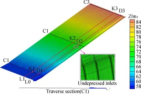
(a)

(b)

There was a rainstorm in Taizhou on July 4, 2012. The rainfall process is shown in Fig.3. The cumulative precipitation reached 71.50 mm, and the maximum rainfall intensity (58.20 mm/h) appeared at 03∶46. Extreme weather has become more frequent in recent years, and the

Tab．2Coordinates and annotations of observation sections

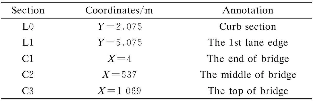
SectionCoordinates/mAnnotationL0Y=2.075Curb sectionL1Y=5.075The 1st lane edgeC1X=4The end of bridgeC2X=537The middle of bridgeC3X=1 069The top of bridge

Tab．3Coordinates and annotations of observation points

PointCoordinates/(m, m)AnnotationD1(4, 2.075)D2(537, 2.075)D3(1069, 2.075)D1, D2 and D3 are the observation points of the ponding at curbK1(4, 5.075)K2(537, 5.075)K3(1069, 5.075)K1, K2 and K3 are the observation points of the lane WFT

natural rainfall intensity has increased significantly[15]. In order to ensure the safety margin of the system, this rainstorm event was chosen as the model dynamic boundary condition.

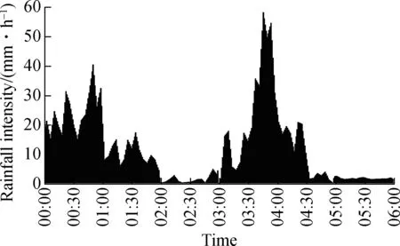
Fig.3 Rainfall intensity on July 4, 2012

2 Results and Discussion

2.1 The temporal distribution

A significantly positive association is observed in Fig.4 between the ponding depth at the curb and the rainfall intensity, while compared to D1 and D2, D3 is clearly lower. Meanwhile, as shown in Tab.4, the maximum ponding depth (29.99 mm) at the curb occurs at 03:49. Fig.5 shows gutter water surface profiles of different transverse sections at 03:49. It illustrates that the ponding width is not constant, and the maximum width is about 1.50 m (from 2.075 to 3.60 m in theXdirection). The shoulder width of the bridge deck is 3.00 m, which indicates that the ponding water does not enter the lanes. Thus, the area above section L1 is the sheet flow, and the sheet flow depth is defined as WFT. The WFT of K1, K2 and K3 also displays a positive relationship with the rainfall intensity (see Fig.6). The WFT of K1, K2 is slightly larger than that of K3, and the maximum WFT (1.64 mm) occurs at 03:47.

Tab.4 gives the specific values of the runoff depth. There is a time interval of 1.00 min with a rainfall intensity of 58.20 mm/h between the peak of the rainfall intensity and lane WFT, which is the sheet flow travel time

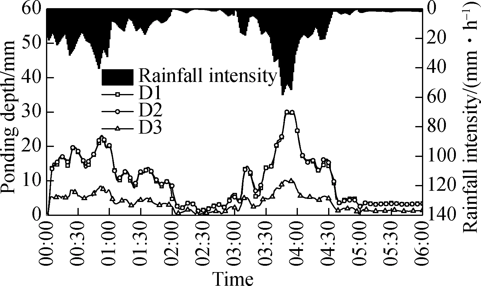
Fig.4 Variation of ponding depth at curb

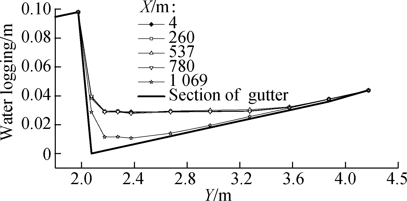
Fig.5 Ponding width at different transverse sections at 03:49

Fig.6 Variation of lane WFT

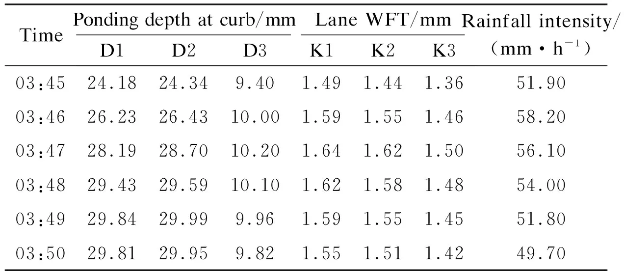
TimePonding depth at curb/mm Lane WFT/mmD1D2D3K1K2K3Rainfall intensity/ (mm·h-1)03:4524.1824.349.401.491.441.3651.9003:4626.2326.4310.001.591.551.4658.2003:4728.1928.7010.201.641.621.5056.1003:4829.4329.5910.101.621.581.4854.0003:4929.8429.999.961.591.551.4551.8003:5029.8129.959.821.551.511.4249.70

for the lane WFT. Hydraulic engineering circular (HEC) 22[16]is widely used in the design of highways and bridges in the US[17]. The sheet flow travel time calculated by HEC-22 method is 1.72 min. The kinematic wave equation with non-optimal coefficients and the simplified momentum equation are used in the HEC-22 method[18], which causes the over-estimation of the sheet flow travel time. According toGeneralSpecificationsforDesignofHighwayBridgesandCulverts(JTG D60—2015)[19]in China, the sheet flow travel time is 1.75 min, which also over-estimates the sheet flow travel time. It is unfavorable to the drainage design of bridge if this time is over-estimated.

We also found that the velocity of the observation points have similar changing laws to the ponding depth at the curb and lane WFT. Thus, this study only presents partial velocity results in Tab.5 and Tab.6, which shows that the velocity and runoff depth reach the maximum value at the same time. The curb obstructs the runoff flow of D1 and D2 in theYdirection. Thus,Vyis close to 0. D3 is the observation point directly above an inlet, the runoff can flow into the inlet, soVyof D3 is not 0. On the other hand, the direction of velocity can be calculated byVy/Vx. Except for D3, the direction of velocity is almost constant with the rainfall intensity changing. Moreover, the velocity direction of D1 is almost the same as that of D2, which also exists in K1, K2 and K3. Meanwhile, since the longitudinal slope is larger than the traverse slope, theVyof K1, K2 and K3 is larger than that ofVx.

Tab．5Velocity of D1, D2 and D3

m/s

TimeD1D2D3VxVyVxVyVxVy03:45-0.750-0.750-0.35-0.0103:46-0.780-0.790-0.37-0.0103:47-0.800-0.810-0.38-0.0103:48-0.820-0.830-0.38-0.0103:49-0.830-0.830-0.37-0.0103:50-0.830-0.830-0.37-0.01

Tab．6Velocity of K1, K2 and K3

m/s

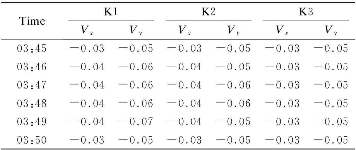
TimeK1K2K3VxVyVxVyVxVy03:45-0.03-0.05-0.03-0.05-0.03-0.0503:46-0.04-0.06-0.04-0.05-0.03-0.0503:47-0.04-0.06-0.04-0.06-0.03-0.0503:48-0.04-0.06-0.04-0.06-0.03-0.0503:49-0.04-0.07-0.04-0.05-0.03-0.0503:50-0.03-0.05-0.03-0.05-0.03-0.05

It is summarized that the ponding depth at the curb, lane WFT and velocity rate are positively related to the rainfall intensity. In order to compare their changes in the time dimension, the variation coefficient of the above three runoff parameters is calculated by

(2)

The value ofCvreflects the response degree of runoff parameters to rainfall intensity. In this study, the change of the above three runoff parameters is caused by the change in rainfall intensity. A smallerCvindicates relatively stable runoff characteristics, and runoff characteristics have a slower response to the rainfall intensity. Conversely, a higherCvindicates that the runoff characteristics are severely volatile and have a faster response to the rainfall intensity.

Tab．7Coefficient of variation of runoff parameters

Observation pointsCoefficient of variation CvD1D2D3K1K2K3WFT0.680.670.68Ponding depth at curb0.710.710.69Velocity rate0.660.660.760.790.790.81Direction of velocity0.050.050.050.180.180.18

It is obvious that theCvof velocity direction is very low, which indicates that the direction of velocity of runoff is relatively stable. The other three are relatively high, they are volatile and have higher research significance. TheCvof WFT(K1, K2 and K3) is lower than that of ponding (D1, D2 and D3). Meanwhile, for the velocity rate, theCvof K1,K2 and K3 is higher than that of D1,D2, and D3. This indicates that the WFT of K1, K2 and K3 has relatively weak variability in the time dimension. However, their velocity rates are more volatile than those of D1, D2 and D3.

The simulation results point out that the temporal distribution of bridge deck runoff is changing in real-time, and the runoff parameters have a positive relationship with rainfall intensity; however, their response degrees to rainfall intensity are different, and there are also spatial differences. Furthermore, the typical methods in specifications lead to an over-estimation on the sheet flow travel time.

2.2 The spatial distribution

In order to explore the spatial distribution laws, the result of section L0 and L1 at 03∶50 is extracted and demonstrated in Fig.7. The direction of runoff velocity is relatively stable. Thus, the direction of velocity is not the key. This study focuses on the ponding depth at the curb, the lane WFT and the velocity rate.

Fig.7 Results of L0 and L1 along with X at 03∶50

Figs.7 and 8 demonstrate that inlets can affect the runoff distributions, and the changes of the runoff distributions keep stable after rainwater concentrates. W1 (544.23, 5.075) is the observation point above the inlet where the minimum lane WFT occurs, and P2 (546, 2.075) and W2 (546, 5.075) are the observation points where the maximum runoff depth occurs. In order to quantify the inlet’s effects on the distribution of bridge deck runoff, the above observation points are extracted to calculate the effect degree.

Fig.8 Spatial distributions of runoff at 03∶50

The velocity of sheet flow is calculated by the Chézy equation and Manning equation:

(3)

(4)

whereVis the velocity of sheet flow, m/s;Cis the Chézy coefficient;Ris the hydraulic radius, m; andJis the hydraulic gradient.

The lane WFT and velocity rate can be comprehensively represented by the unit discharge of sheet flowQu(m3/s):

(5)

For the sheet flow,Ris the lane WFT, andJis the slope of bridge deck.

When two observation points have the sameYcoordinates, their unit discharges are equal if there are no inlets on the curb. However, due to the effect of the inlets, their unit discharges are different, and the effect degree of inlet on lane water filmmf(%) is

(6)

where {X1,Y} and {X2,Y} are the coordinate of observation points;h{X1,Y}andh{X2,Y}are the lane WFT of points, m. In this paper, the two points are W1 and W2, respectively.

The ponding depth at the curb and the velocity rate can be comprehensively represented by the gutter discharge. In accordance with HEC-22 and Schalla’s study[20], the interception efficiency of the inlets is a perfect parameter to evaluate the inlet’s influence on the ponding at the curb:

(7)

(8)

(9)

wheremdis the effect degree of inlet on the ponding at curb, %;nis the Manning coefficient;SLis the longitudinal slope;Sxis the transverse slope;ypis the ponding depth at the curb, m, in this paper,ypis the ponding depth of P2.Qais the gutter flow, m3/s;LTis the curb opening length required to intercept 100% of the gutter flow, m;Lis the curb opening length, m, and in this paper,L= 0.35 m.

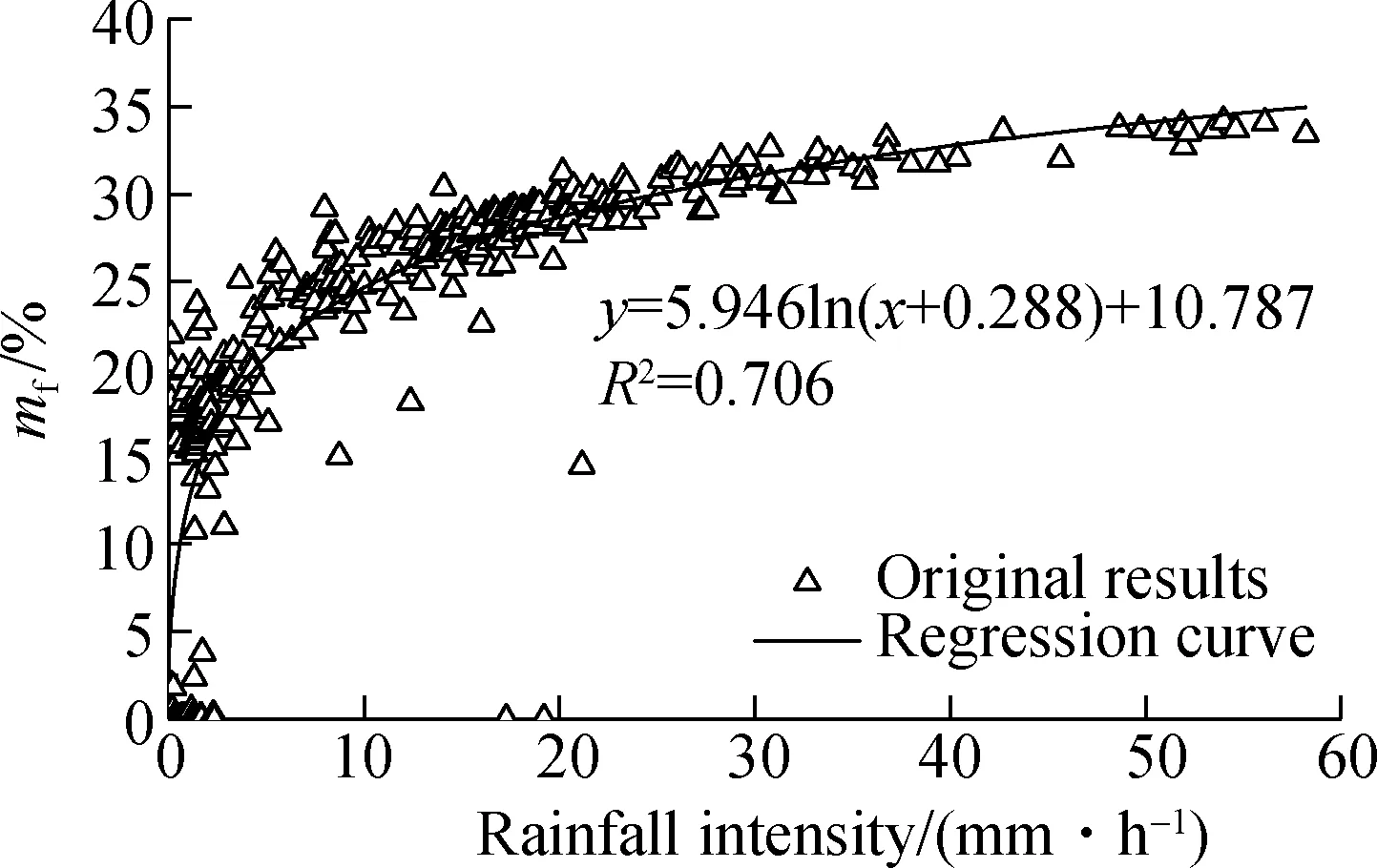
Using Eq.(6) and Eq.(9),mfandmdcan be calculated. From the comparison in Fig.9,mfhas a positive relationship with rainfall intensity; whenmdis opposite, the relationship is negative.

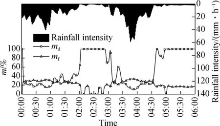
Fig.9 Variations of md and mf along with time

Based on a large amount of objective data, the regression method is the most representative and it is widely applied when exploring the related law among different parameters. Consequently, it is also used to reflect the trends ofmdandmfwith the changes of rainfall intensity. Fig.10 illustrates thatR2(goodness-of-fit) is 0.824 formd, andR2is 0.706 formffor Taizhou Bridge. During a natural rainstorm process, the inlet’s effects on lane WFT and the ponding depth at the curb have a nonlinear quantitative relationship with the rainfall intensity.

2.3 Characteristics of bridge approach slab runoff

At the end of bridge, the bridge approach slab is designed for the transition ofSLto prevent bumping. Bridge approach slab runoff is heavy for large span bridges after the rain concentrates. Accordingly, bridge approach slab will come under obvious attack. Ponding with a larger area is one of the significant impacts whenSLdecreases.

(a)

(b)

In this simulation, the bridge approach slab is divided into three transition segments (from 0 to -15 m in theXdirection) andSLranges from 2.5% to 0%. T1, T2 and T3 sections in Fig.11 are used to analyze the runoff distribution with the change ofSL.

Fig.11 Flow field of bridge approach slab runoff at 03∶49

As depicted in Fig.11, the streamline field presents a slight change, but it is dramatic at -15 m ofX, which indicates that streamline field of bridge approach slab runoff is not sensitive to the change ofSL, but it rapidly changes at the section with the minimumSL.

As shown in Fig.12, the ponding depth at the curb (T3) continues to increase from 0 to -15 m in theXdirection, especially at the first three slope transition sections, and the rising trend is sharp. Then, the ponding depth at the curb decreases close to -15 m ofXdue to a large inlet. The results indicate that the ponding depth at curb is significantly sensitive to the change ofSLand increases from 30.12 to 58.14 mm. Thus, an effective

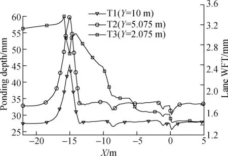
Fig.12 Runoff depth at 03∶49 with variation of T1, T2 and T3

drainage design is necessary at the bridge approach slab. On the other hand, the lane WFT (T1 and T2) only has a precipitous change near -15 m ofX, and the maximum lane WFT is 3.26 mm, which indicates that lane WFT is sensitive to the location with the minimumSL. Except for the zone of sudden change, the lane WFT changes little; the lane WFT of T1 is about 1.25 mm; and that of T2 is about 1.61 mm. Thus, the lane WFT is insensitive to the gradual change ofSL, which is consistent with the conclusion of Ref.[4].

3 Conclusions

1) The runoff depth and velocity rate show a positive relationship with the rainfall intensity; however, there are some differences in their response degrees to it. The obvious spatiotemporal differences are shown in the characteristics of bridge deck runoff.

2) With the change in the rainfall intensity, the inlet’s effect degree on lane water film can be described as a natural logarithm function (R2=0.706). Yet, the inlet’s effect degree on the ponding at the curb can be illustrated as a negative exponential function (R2=0.824). The inlet’s effects on bridge deck runoff show a good quantitative relationship with the rainfall intensity.

3) At the bridge approach slab, the lane WFT is insensitive to the change ofSL, but it significantly increases at the location with the minimumSL. Conversely, the ponding depth at the curb is very sensitive to the change ofSL. The effective drainage measures are necessary, and the location with the minimumSLneeds to be paid sufficient attention at the bridge approach slab.