Xi-chen Wang (王希晨), Jian Zhang (张健), Xiao-dong Yu (俞晓东), Sheng Chen (陈胜)

College of Water Conservancy and Hydropower Engineering, Hohai University, Nanjing 210098, China

Abstract: The vent tube is commonly used for the water hammer protection in the hydropower tailrace system. In transient processes,with air entering and exiting the vent tube, one sees complex hydraulic phenomena, which threaten the station’s safe operation. It is necessary to investigate the transient mechanisms in the tailrace system with vent tube. In this paper, a 3-D, two-phase numerical model of a vent tube on the connection of the tailrace tunnel and the diversion tunnel, is developed based on the FLUENT with the volume of fluid (VOF) algorithm to investigate the transient air-water flow patterns and the complex hydraulic phenomena in the vent tube of the tailrace system. A 1-D and 3-D unidirectional adjacent coupling (1-D-3-D-UAC) approach with a linear interpolation method is adopted to adjust the timesteps between the 1-D model and the 3-D model on the tunnel inlet and outlet boundaries through the user defined function (UDF), to transmit the data from the 1-D model to the 3-D model. The model is verified by comparing the results obtained by using the 1-D model alone and from the experiments in literature. The transient flow processes under the full load rejection consist of four stages: the water level dropping stage, the air entering stage, the air pocket collapsing stage, and the air exiting stage.Detailed hydraulic phenomena in the air pocket collapsing process are also discussed.

Key words: Vent tube, tailrace tunnel, two phase, volume of fluid (VOF), 1-D-3-D coupling

Introduction

In the later stage of the construction of a large diversion type hydropower station, the diversion tunnel with a high bottom elevation is normally connected with the tailrace tunnel in view of the construction economy. When a hydropower station works in transient processes such as in the load rejection process, the air may accumulate in the high parts of the tailrace system when the pressure reduces to the vaporization level to form an air pocket, which is known as the liquid column separation. When the trapped air pocket collapses, the pressure increases in a great extent. The free-surface-pressure flow and the intense pressure pulsation become potential dangers to the safe operation of the hydropower station. Thus, the vent tube, as a common measure to regulate the pressure in engineering projects, is usually set on higher parts of the tailrace system, often on the connection of the tailrace tunnel and the diversion tunnel, to allow the air to pass through to relieve the transient pressure, so that the operation risks could be reduced[1]. Zhang et al.[2]carried out a series of model tests to support this approach. However, with the air entering and exiting the vent tube, the hydraulic phenomena in the tailrace system become very complex. Therefore, it is important to investigate the transient mechanisms and the detailed behaviors of the two-phase flow in the tailrace system with the vent tube, as is important for the engineering design and the hydraulic protection. However, the air entering and exiting processes and the complex two-phase flow phenomena in the vent tube in the hydropower tailrace system remain not well studied so far.

The hydraulic transients in a tailrace system were studied by numerical methods in view of convenience and economy. The method of characteristics (MOC) is applied, as a mature and reliable methodology with advantages of accuracy and convenience in the 1-D numerical calculation of hydraulic transient pro-blems[3-6]. However, the MOC has defects in applications in multi-dimensional fields. With the development of computer science, the computational fluid dynamics (CFD) has been developed and widely used in many fields, including water conservancy engineering researches[7-11], for its advantages in obtaining multi-dimensional fluid flows in required details. Thus,in order to study transient processes in the hydropower tailrace system in a 3-D perspective, the CFD method was adopted. Nevertheless, the CFD method is not suitable for large scale calculations with a large number of computational grids, because of limitations of computing resources. Hence, the MOC and the CFD methods were combinded together with boundary interfaces between 1-D and 3-D models[12-17].Zhang et al.[16]proposed two validated 1-D-3-D coupling methods, i.e. the partly overlapped coupling(POC) method and the adjacent coupling (AC) method,where the bidirectional data transmission is adopted,with the advantage of double accuracy. However, the flexibility of the coupling methods with bidirectional transmission is reduced due to the requirement of the same timestep for the two models. In the present paper,a 1-D-3-D unidirectional adjacent coupling (1-D-3-DUAC) method is employed for its flexibility and independence. The boundaries of two models are adjacent and the time-variant data are transmitted from the 1-D model to the 3-D model in one-way. A linear interpolation method is applied on the boundary interfaces, allowing the 3-D model to use a different timestep from that of the 1-D model.

In this paper, in order to investigate the transient air-water flow patterns and the complex hydraulic phenomena in the vent tube of the tailrace system, a 3-D, two-phase flow numerical model with a vent tube on the connection of the tailrace tunnel and the diversion tunnel in a hydropower station is built in full scale. The present 3-D model uses the data output from the 1-D model as the boundary input data on both ends of the tunnel domain. The interfaces between the 1-D and 3-D models are dealt with through a user defined function (UDF) code with a linear interpolation method to adjust the timestep differences between the two models. The results of the 1-D-3-D-UAC model and the 1-D model alone are compared. The transient air-water flow processes generally consist of four stages: the water level dropping stage, the air entering stage, the air pocket collapsing stage, and the air exiting stage. And detailed hydraulic phenomena are revealed.

1. Numerical model setup

1.1 Model description

This numerical model, as a part of the tailrace system in a diversion type hydropower station, has a vent tube on the connection of the tailrace tunnel and the diversion tunnel in full scale. The arrangement of the tailrace system and the operating parameters of the units were described in detail in the reference paper[1].Figure 1 shows the simulation domain consisting of a 103 m long pipe as the diversion tunnel connected with a 30 m long changing diameter pipe as the tailrace tunnel in X-direction and a 40 m long pipe as the vent tube on the connection in Z-direction.The inlet diameter of the tailrace tunnel is 18.2 m, and the outlet diameter of the diversion tunnel is 20.7 m.The bottom elevations of the tailrace tunnel and the diversion tunnel are both 361.3 m. The diameter of the vent tube is 3.3 m. The gravity is set along the negative Z-direction. The domain is meshed into 358 548 cells, with a refinement in the T-junction area.

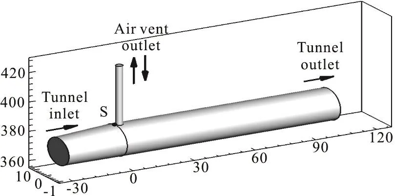
Fig. 1 Simulation domain (m)

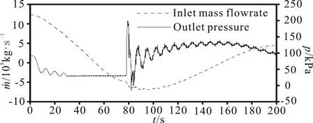
Fig. 2 Transient input data of 1-D-3-D-UAC model

A non-slip boundary condition is applied on all pipe walls. There are one inlet boundary set with the mass-flow-inlet and two outlet boundaries set with the pressure outlet (as shown in Fig. 1). The tunnel inlet is set with an initial water mass flowrate of 1 227 074.5 kg/s(without air entering the tunnel), the tunnel outlet is set with an initial average gauge pressure of 92 036.4 Pa(with a correction factor applied to the pressure output from the 1-D model in order to reduce the impact of the back flow from the outlet boundary of the 3-D model) and the vent tube outlet is set to the atmospheric pressure. A UDF code is developed on the tunnel inlet and outlet boundaries to allow the time-varying data to transmit from the 1-D model to the 3-D model in only one direction. 200 s long data obtained by using the 1-D model alone, which simulates the transient processes in the tailrace system under the full load rejection condition[1], are selected as the input parameters of the 1-D-3-D-UAC boundaries. The transient input data of the tunnel inlet and outlet in the 3-D model are shown in Fig. 2, in which m˙ stands for mass flowrate, t stands for time and p stands for pressure.

1.2 Methodology

The present 1-D-3-D-UAC model is built based on ANSYS FLUENT 15.0, which is a powerful and widely used CFD software. The volume of fluid (VOF)method is employed to simulate the two-phase flow patterns for its advantageous ability of tracking the gas-liquid interface. The realizable k-ε model is selected for higher accuracy to simulate the turbulent flow, and the standard wall function is applied for the fluid in the proximity of the walls.

In this model, the air is treated as the primary phase, and the liquid water is treated as the secondary phase. The mass and heat transfers between the two phases are not considered. The continuity equation is as follows

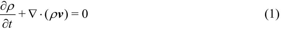
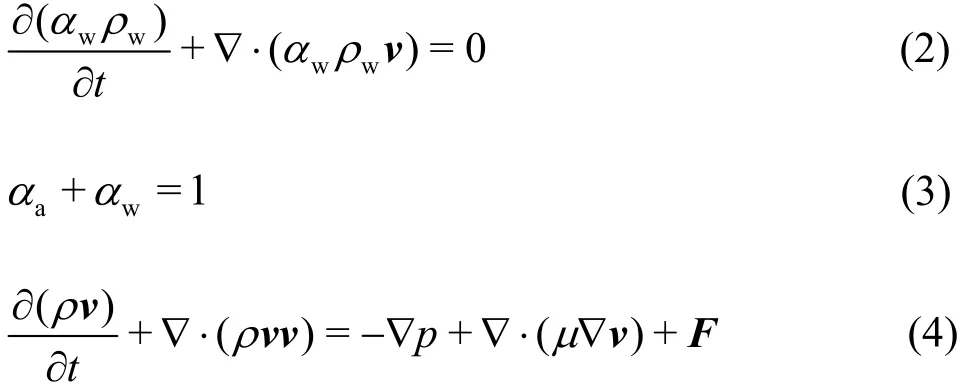
To track the air-water interface, the continuity equation for the volume fraction of the liquid water is solved through Eq. (2), and then the volume fraction of the air is calculated based on Eq. (3). A single momentum equation expressed as Eq. (4) is used since the air and the liquid water share the same velocity fields[18]. In the following equations, α is the volume fraction, ρ is the density, with the subscripts w denoting the liquid water and a the air,μ is the kinematic viscosity, and F stands for the mass force.

In order to obtain the initial flow field with a clear air-water interface, the explicit scheme, as a time-dependent solution, is implemented from the beginning. In other words, the numerical model is used in the calculation under the initial condition by the unsteady solver for a period of time until the monitoring parameters become basically stable, and then with the simulation results, treated as the initial flow field, the calculation continues when the UDF code of the 1-D-3-D-UAC method is implemented on the boundaries.

A 1-D model simulating the transient processes in the tailrace system with vent tube was developed,by Yu et al, in the FORTRAN language, based on the MOC and the discrete free-gas cavity model (DGCM).The detailed methodology of the 1-D model is found in Ref. [1].

1.3 1-D-3-D unidirectional coupling method

The schematic diagram of the 1-D-3-D-UAC method is presented in Fig. 3. Point A in the 1-D model corresponds to the inlet of the tailrace tunnel in the 3-D model, and Point B corresponds to the outlet of the diversion tunnel. The 1-D model of the entire tailrace system is applied firstly[1]. The mass flowrate at Point A and the pressure at Point B obtained with the 1-D model are stored in a data file. A UDF code file is implemented on the inlet and the outlet boundaries of the 3-D model as the interfaces,respectively, feeding the 1-D data to the 3-D model during the calculations. The data transmission on the two boundaries is unidirectional, from the 1-D model to the 3-D model.

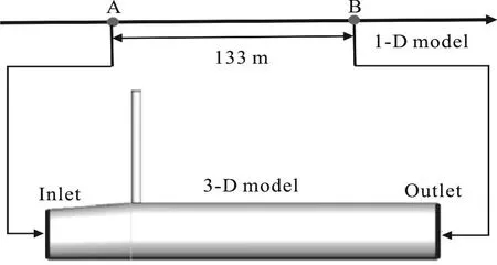
Fig. 3 Schematic diagram of 1-D-3-D-UAC method

By the implementation of the 1-D-3-D-UAC method, the timestep of the 3-D model is not necessarily equal to that of the 1-D model. A linear interpolation method, described in Eq. (5), is employed to deal with the difference of the timestep intervals between the 1-D model and the 3-D model.

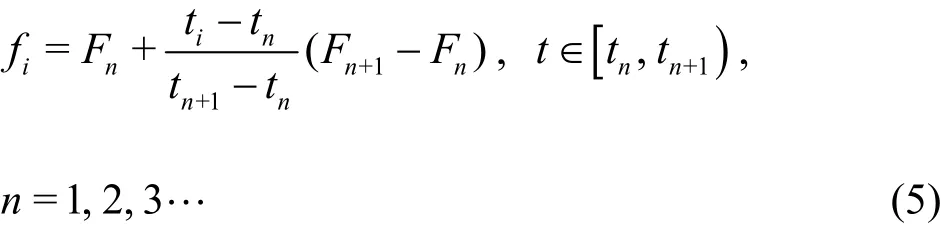
In Eq. (5), Fnand Fn+1are two adjacent data obtained with the 1-D model corresponding to timetnand tn+1, respectively, and fiis the input parameter on the boundaries of the 3-D model at the current computational time ti.

2. Results and discussions

2.1 General transient processes

Figure 4, in whichwα stands for the volume fraction of water, including a series of 3-D phase contour images withwα under 0.45 cut off for a clearer presentation at several selected time points,generally shows the entire transient processes in the vent tube on the connection of the tailrace tunnel and the diversion tunnel under the full load rejection condition. The general transient processes consist of four stages: the water level dropping stage, the air entering stage, the air pocket collapsing stage, and the air exiting stage.

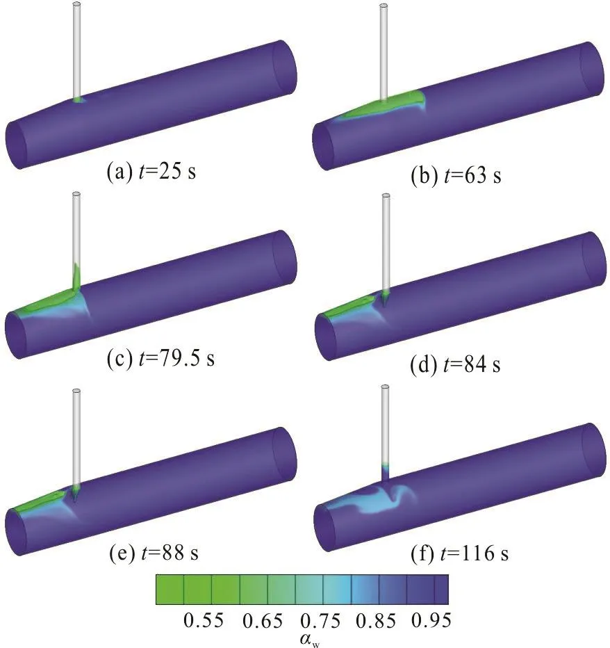
Fig. 4 (Color online) General transient processes under full load rejection condition

(1) Stage1: Water level dropping

After the full load rejection, the water level drops rapidly in the form of fluctuations in the vent tube.When it reaches the top of the tunnel, a small amount of air is sucked into the tunnel (Fig. 4(a)), as mentioned in the reference paper[1], which cannot be captured by the 1-D model alone.

(2) Stage 2: Air entering

With the water level falling under the bottom plane of the vent tube, the air enters the tunnel and an air pocket forms and extends along the upper wall of the tunnel to both sides. Then the edge of the air pocket in the diversion tunnel is blocked by the reversed flow and squeezed backward (Fig. 4(b)).

(3) Stage 3: Air pocket collapsing

The air pocket collapses with the water impacting on the lower part of the vent tube wall, and a huge impact pressure is generated. The water drives part of the air into the vent tube (Fig. 4(c)) with the rest still trapped in the tailrace tunnel. The water level in the vent tube rises rapidly due to the water hammer and declines sharply due to the reflection (Fig. 4(d)). The air enters the tunnel by the fluid inertia and merges with the air trapped before. Repeatedly, the water drives the air into the vent tube and then drops back into the tunnel (Fig. 4(e)).

(4) Stage 4: Air exiting

The residual air in the tunnel is discharged through the vent tube gradually with the water entering and exiting the tunnel (Fig. 4(f)).

2.2 Comparisons of model results

The comparison of the water level histories between the results obtained by using the 1-D-3-D-UAC model and the 1-D model alone is shown in Fig. 5, in which H stands for water level, while the comparison of the pressure histories at the front bottom of the vent tube (Point S in Fig. 1) is shown in Fig. 6.The dashed curve represents the data obtained by the 1-D model alone and the solid one represents those obtained by the 1-D-3-D-UAC model.

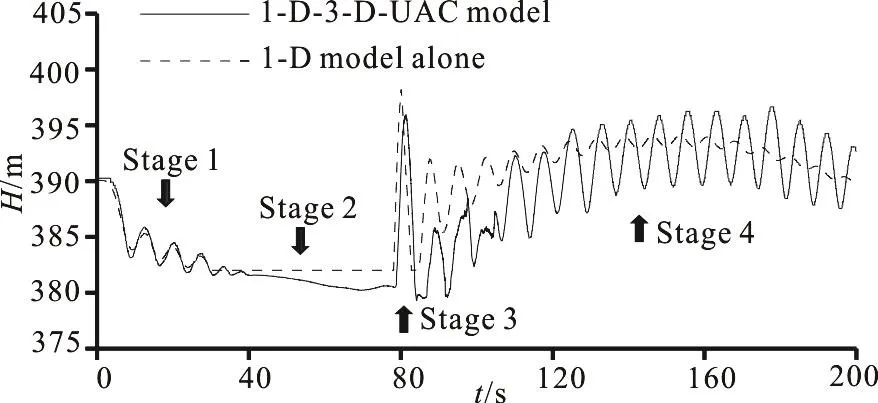
Fig. 5 Comparison of water level changing histories

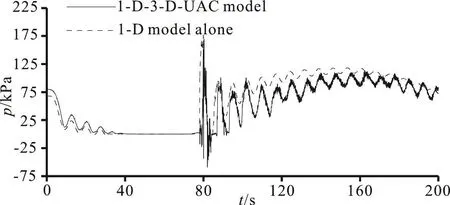
Fig. 6 Comparison of pressure changing histories at the vent tube front bottom

As mentioned in Section 2.1, the entire transient processes consist of four stages. In stage 1, the variation curves of the water level and the pressure obtained by the 1-D-3-D-UAC model and by the 1-D model alone agree well with each other, except that there is a minor difference in the initial pressure and the fluctuation obtained by the 1-D-3-D-UAC model in stage 1 lasts longer. The initial difference, which leads to differences in the fluctuation amplitudes in stage 3 and stage 4, may be due to the unavoidable backflow at the outlet boundaries, as generally exists in multi-dimensional CFD models and simplified boundary conditions with the 1-D model. In stage 2,the pressures obtained by both models stay zero, but the water level obtained by the 1-D-3-D-UAC model drops slowly while that obtained by the 1-D model alone stays horizontal due to different air-water interface tracking methods in the two models. With the 1-D-3-D-UAC model, the change of the water level is monitored by tracking the area-weighted height of an isosurface with a volume fraction of water equivalent to 0.5 in both the vent tube domain and the tunnel domain, and the air-water interface is free depending on specific flow patterns. In contrast,with the 1-D model alone, the change of the water level is just computed in the vent tube while that in the tunnel domain is ignored, and the air-water interface is assumed to be flat and complete in movements.Moreover, the discharge coefficient of the vent tube is set to be constant in the 1-D model rather than changing as in reality, and the flow inertia is not considered either. Therefore, a slight time lag occurs with the 1-D-3-D-UAC model, and one sees obvious differences in the peak, the amplitude and the smoothness between the results obtained by the two models in stage 3 and stage 4. By zooming the pressure curve in stage 3 in Fig. 6 to see the air pocket collapsing process (Fig. 7), it can be noticed that the curve obtained by the 1-D-3-D-UAC model changes greatly with a poor smoothness, and small fluctuations appear around zero when the water level drops under the upper ceiling of the tunnel after the first collapse.The waveform in stage 3 obtained by this model is similar to the experimental results from Zhang et al.(Fig. 4 in Ref. [2]).

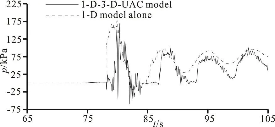
Fig. 7 Comparison of pressures at the vent tube front bottom in the air pocket collapsing process

Figure 8 shows the air volume flowrate (denoted by Qa) through the bottom plane of the vent tube over time obtained by the 1-D-3-D-UAC model. The flow direction from the vent tube to the tunnel is taken as the positive direction and the reverse flow direction is the negative direction. The subgraph of Fig. 8 displays the results obtained by the 1-D model alone(Fig. 6 in Ref. [1]) with the black solid line standing for the velocity of the air (denoted by va) travelling through the vent tube of the same diameter. The shapes of the curves between the two models are similar. By contrast, with the 1-D-3-D-UAC model,the air flow changes more sharply, and attenuates quickly in the air pocket collapsing process, maybe due to different air-water interface tracking methods mentioned above.

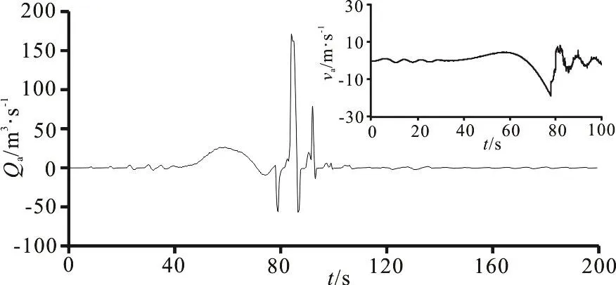
Fig. 8 Air volume flowrate through the vent tube bottom plane obtained by the 1-D-3-D-UAC model (Subfigure: air velocity in vent tube obtained by the 1-D model alone[1])

Despite some differences between the results obtained by the 1-D-3-D-UAC model and the 1-D model alone, the variations have the same trend, in agreement with the results of experiments conducted by other researchers. Therefore, to a certain extent, the present model is verified.

2.3 Hydraulic phenomena in air pocket collapsing process

Among the four stages mentioned above, stage 3,i.e., the air pocket collapsing process is the most noteworthy because of its most complex hydraulic characteristics and the great pressure transients.

For better understanding the physical nature, a series of pictures showing the water volume fraction contours and the corresponding pressure and velocity distributions on the locally zoomed X-Z plane at Y=0 m in the air pocket collapsing process are presented in Fig. 9. The pressure in the tunnel is greatly relieved as the air enters from the vent tube,and increases rapidly as the water runs into the vent tube (Figs. 9(a), 9(b)). It can be noticed that, when the water driven by the impact force of the air pocket collapsing enters the vent tube, it first hits the lower part of the vent tube wall on the tailrace tunnel side and climbs rapidly along the wall (Figs. 9(b1), 9(d1)),with the pressure increasing greatly and with a low pressure zone forming on the other side of the wall(Fig. 9(b2)). The water with air in it, rises with the broken and unclear interface, leading to a water spray,or named as “geysering”[19-21]. When the water level drops under the upper ceiling of the tunnel because of the reflection of the water hammer and the flow inertia(Fig. 9(c1)), a low pressure zone appears on the top of the joint of the tailrace tunnel and the diversion tunnel(Fig. 9(c2)), or the diameter changing area, and causes a bottom-up vortex (Fig. 9(d1)).

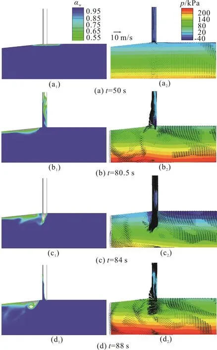
Fig. 9 (Color online) Flow patterns in the air pocket collapsing process with corresponding pressure and velocity distribution

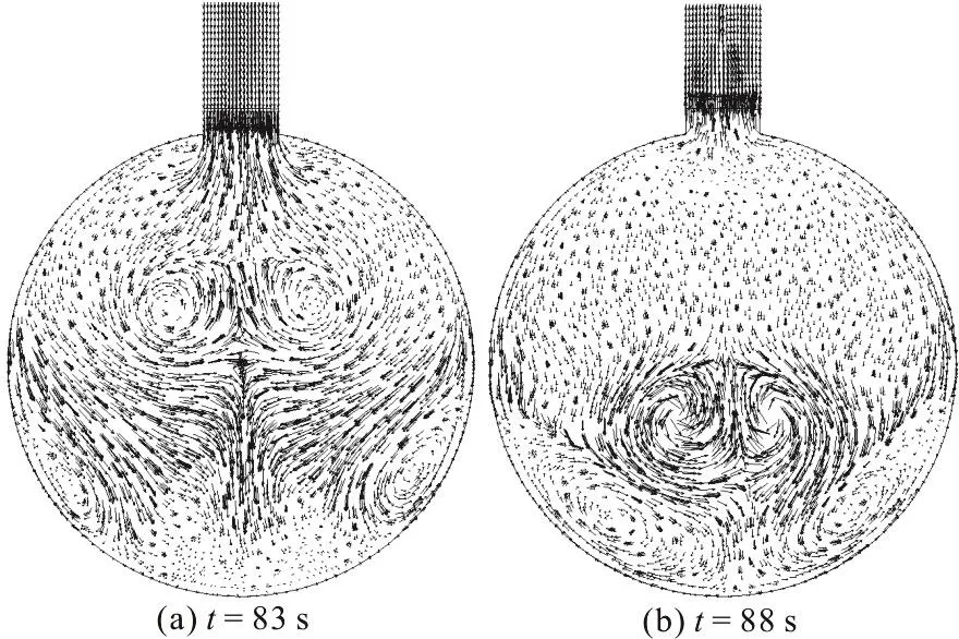
Fig. 10 Symmetrical vortices in tunnel bottom in the air pocket collapsing process

The velocity field on the Y-Z plane extracted at X=0 m is plotted with a uniform vector length at t=83s and t=88s in Fig. 10, where it is shown that the vortices are in an approximate symmetrical distribution, mainly in the lower part of the tunnel,when the water goes in (Fig. 10(a)) and out of the tunnel (Fig. 10(b)) in the air pocket collapsing process.

3. Conclusions

The transient air-water flow patterns in the vent tube of the tailrace system in a diversion type hydropower station is investigated by developing a 3-D, two-phase and unsteady numerical model. The 1-D-3-D unidirectional adjacent coupling (1-D-3-DUAC) approach is implemented on the inlet and outlet boundaries of the tunnel through a user defined function (UDF) code, and verified by comparing its results with those obtained by using the 1-D model alone and by experiments already conducted by other researchers. The entire transient air-water flow processes under the full load rejection are studied. Some conclusions are as follows:

(1) The coupling of the 1-D and 3-D models combines the advantages of two models and can greatly save computational resources and better depict the flow patterns. The implementation of the unidirectional adjacent coupling approach allows the 3-D model to take its boundary inputs provided by the 1-D model. The linear interpolation method enables the two models to calculate with different timesteps.Therefore, the present 1-D-3-D-UAC model, with its advantages of flexibility and independence, can become an effective scientific tool in the research for the long-distance water hammer protection.

(2) The entire transient air-water flow processes in the vent tube of a hydropower tailrace system under the full load rejection condition are divided into four stages: the water level dropping stage, the air entering stage, the air pocket collapsing stage and the air exiting stage.

(3) In the water level dropping process and the air entering process, the air goes into the tunnel through the vent tube, and the pressure in the tunnel is greatly relieved to form an air pocket.

(4) In the air pocket collapsing process, the water drives air into the vent tube, causing huge impact pressures. Some hydraulic phenomena, including the water spray, the low pressure zones, the symmetric vortices and the negative pressure oscillations, happen in this process.

(5) The vent tube is an effective measure to adjust the pressure in transient processes; however,the air entering and exiting the vent tube brings about intense pressure fluctuations and complex hydraulic phenomena, threatening the safety of operation.

The analyses of the transient air-water flow processes and the detailed hydraulic phenomena by using the present 1-D-3-D-UAC model provide some fundamental understanding for the study of transient mechanisms and the design and optimization of the vent tube in the hydropower tailrace system. In the future, a model experiment will be conducted to further validate the present numerical model, and the verified 1-D-3-D-UAC model will be implemented in the follow-up studies of the vent tube and other hydraulic transient protections.