Mohammad Mahdi Jalali, Alistair G. L. Borthwick

Institute for Energy Systems, School of Engineering, The University of Edinburgh, Edinburgh, UK

Abstract: A model is presented of particle advection near groynes in an open channel. Open channel hydrodynamics is modelled using the shallow water equations, obtained as the depth-averaged form of Reynolds-averaged continuity and Navier-Stokes momentum equations. A Lagrangian particle-tracking model is used to predict trajectories of tracer particles advected by the flow field, with bilinear interpolation representing the continuous flow field. The particle-tracking model is verified for chaotic advection in an alternating flow field of a pair of blinking vortices. The combined shallow flow and Lagrangian particle-tracking model is applied to the simulation of tracer advection in flow past a pair of side-wall cavities separated by a groyne, and in an open rectangular channel containing a pair of parallel groynes oriented normal to the channel wall. The study is potentially useful in understanding mixing processes in shallow flow fields near hydraulic structures in wide rivers.

Key words: Shallow water equations, Lagrangian particle tracking, chaotic advection, blinking vortices, side-wall cavities, groynes

Introduction

Mixing occurs due to advection and dispersion processes whereby species become distributed within a flow field[1]. Mixing processes are promoted by shear in a shallow flow primarily through vorticity from eddies, and directly influence the transport of material, heat, and contaminants, thus affecting water quality. In laminar flow, diffusion is entirely due to molecular processes, and follows Fickʼs Law whereby the rate of mass transfer of a substance per unit area is proportional to the concentration gradient. In turbulent flow, the diffusing substance is transferred by turbulent fluctuations as well as by molecular diffusion, and,by analogy with Fickʼs first law, it may be assumed that the turbulent flux is proportional to the gradient of the time-averaged concentration[1]. An important factor in river mixing processes is the presence of large-scale turbulent eddies, which may be created from the bed boundary layer as it rolls up into vortices,and from flow separation at obstacles and side wall boundary layers, such eddies play a major role in entraining sediment into suspension and driving sediment transport in a channel. In rivers with erodible beds, the flow hydrodynamics alters the channel morphology and mixing processes, thus affecting water quality. Ongoing advances in computer power and improved mathematical modelling of shallow flows have enabled numerical simulation techniques to be used increasingly to model water and sediment flows and mixing processes in open channels.

Lagrangian particle tracking is of great use in investigating dispersion processes in advection-dominated flow fields. The seminal work on chaotic advection of particles is due to Aref[2]who examined the very complicated trajectories of particles in the simple, but abruptly alternating flow field of a pair of blinking vortices. Aref discovered that the particle trajectories altered from periodic to chaotic as the stirring strength increased, and used stroboscopic maps (i.e., snapshots of particle positions at periodic intervals, where the period matches the blinking period of the vortices) to visualise the influence of stirring period on the tendency towards chaos.Kranenburg[3]considered the wind-induced chaotic advection of particles in a closed circular dish-like basin, where the wind direction changed periodically,and the flow field alternated abruptly. Kranenburgʼs model used a theoretical stream function distribution that fitted the solution to the shallow water equations to estimate the steady-state, wind-induced, depthaveraged velocity field in a circular basin. Although the velocity field is not realistic – depth-averaging obscures 3-D flow processes in this case. The progress from periodic to chaotic advection is remarkably similar to that obtained by Aref for the blinking vortex problem, noting that in Kranenburgʼs case the wind strength replaces the stirrer strength as the governing parameter.

There are many examples of the use of particle tracking to study contaminant dispersion in shallow flows. Pearson and Barber[4]applied Lagrangian particle tracking to simulate the dispersion of coastal pollutant by solving an advection-diffusion equation on orthogonal boundary-fitted grids. Weitbrecht et al.[5]used 2-D particle tracking to examine 1-D advection-diffusion equation in a river, and validated their model against laboratory measurements of flow in a rectangular open channel with groynes. In a study that is particularly relevant to the present research,Zsugyel et al.[6]utilised particle tracking and meticulous laboratory measurements to investigate mixing processes in the vicinity of a single groyne in a rectangular channel. Zsugyel et al. examined the nonlinear characteristics of the particle trajectories,and presented information on flushing times, particle escape rates, mixing processes (through Lyapunov exponents), and the presence of Lagrangian coherent structures, chaotic saddles, and fractal dimensions.The advection and dispersion of sediment particles is particularly complicated in shallow flow fields near groynes and other hydraulic structures introduced into rivers for control purposes. Field observations, laboratory studies, and numerical simulation all offer insights into advection and mixing processes in open channels[7]. The resulting knowledge is useful to hydraulic engineers charged with designing works to control flood flows, protect riverbanks against erosion,and optimize flood protection works.

This paper introduces a coupled numerical solver of the shallow water equations with Lagrangian particle tracking, aimed at studying the chaotic advection of particles near groynes in open channels.The shallow water equations are discretised in space using central differences and the solution marched forward in time using 4th-order Runge-Kutta time integration. The Lagrangian particle-tracking scheme involves integrating the pure advection equation forward in time, again using a 4th-order Runge-Kutta scheme, and is verified against Arefʼs[2]analytical solution for chaotic advection in the flow field of a pair of blinking vortices. The coupled shallow flow and particle-tracking model is then used to simulate chaotic advection and mixing processes in a channel containing a pair of side-wall cavities containing a single groyne, and a rectangular channel containing a pair of groynes.

1. Shallow water equations

The 2-D shallow water equations apply to nearly horizontal flows in wide, open channels, rivers, and lakes. The shallow water equations may be derived in several ways, including: depth-averaging of the 3- D Reynolds-averaged continuity and Navier-Stokes momentum equations obtained from mass and momentum balances across a small control volume[8], and control volume analysis of elements that extend through the depth, with velocity assumed uniform in the vertical direction[9]. After integration of the Reynolds-averaged continuity and Navier-Stokes momentum equations over the depth from the bed at z=-hsto the free surface at z=ζ, and applying suitable boundary conditions at the bed and free surface, the shallow flow equations are as follows:

and

in which U and V are the depth-averaged velocity components in the Cartesian x, y directions, t is time, h is total depth (h=hs+ζ), f is the Coriolis coefficient, g is the acceleration due to gravity, ρ is the density of water, τwxand τwyare the wind stress components in the x- and ydirections, τbxand τbyare the bed stress components in the x- and y-directions, Txx, Txyand Tyyare the effective stresses, and β1, β2and β3are momentum correction factors.

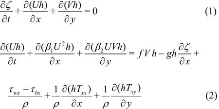
Equations (1)-(3) are discretized using secondorder finite differences[7,10-11]. The numerical solution is then obtained using an explicit time marching scheme based on the 4th-order Runge-Kutta method.In this case, the grid is rectangular, such that x=iΔ x and y=jΔ y, where i=1,2,…imaxand j=1,2,… jmaxare indices and Δx and Δy are grid intervals in the x- and y-directions. Time is set such that t=kΔ t.

2. Lagrangian particle tracking scheme

Lagrangian particle tracking is used to predict the trajectories of tracer particles, with bilinear interpolation providing a representation of the continuous flow field obtained from the discrete results on the numerical grid used by the shallow flow solver[7]. In a fluid flow, the advection of a tracer is described by:

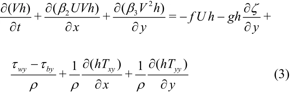
where (up,vp) are the Cartesian velocity components of a particle located at (xp,yp). For a passive tracer the particle velocity at a point in space and time is the same as the flow velocity there. The Lagrangian particle tracking-scheme is developed by integrating the advection equations (4) forward in time using a 4th-order Runge-Kutta time integration method as follows:

where

21.Made a present of these to the king: Gift giving has long been a method of gaining favor, such as with a king. Gifts are often presented to sovereigns, dignitaries, and diplomats in hopes of gaining their favor while showing honor to them. Gift giving can also be used to show one s wealth through the costliness of the gift.

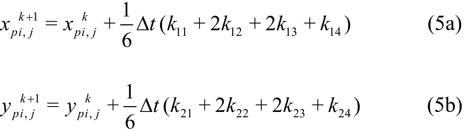
In cases where the velocity field is known analytically as a continuous function, we simply set (up(xp,yp,t),vp(xp,yp,t))=(u( xp,yp, t), v( xp,yp, t))where u and v are the flow velocity components. In cases where the velocity field is computed at discrete points on a grid, the particle velocity is calculated using bilinear interpolation[7]. The interpolation process involves three stages. First, the cell containing the particle is identified as i=ipand j=jpwhen xi＜xp＜xi+1and yi＜yp＜yi+1. We then determine (u1, v1) at the south side of the cell at a position aligned with(xp,yjp) as follows:

and

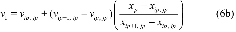
And we next determine (u2, v2) at the north side of the cell at a position aligned with (xp,yjp+1)as follows:

and

The third step involves interpolation in the ydirection, giving (up,vp) as:

Fig. 1 Analytically predicted stroboscopic maps of particles in the flow field induced by a pair of blinking vortices[2]

and

3. Model verification for chaotic advection due to a blinking-vortex pair

The first vortex is centred at (x1, y1)=(-0.5,0) and the second vortex at (x2,y2)=(0.5,0). The blinking vortex model operates by switching on the first vortex,with the second off, for half a cycle during nT＜t＜nT+T/2 where n=0,1,2… and T is the prescribed cycle period. The flow field is abruptly switched at t=nT+T/2 so that the second vortex is turned on while the other one is off during the latter half of the cycle when nT+T/2＜t＜(n+1)T. The process is repeated for n=0,1,2…until the simulation is complete.

Aref[2]defines a dimensionless parameter μ as follows

where T is the blinking period, Γ is the vortex strength, and a is the distance of the centre of the blinking vortex from the origin. By setting Γ=2π and a=1, the dimensionless parameter μ is equal to the period T. The choice of value for μ has a profound effect on thelong-term dynamic behaviour of particles.FollowingAref[2], we considerblinking vortices located at (x1, y1)=(-0.5,0) and (x2,y2)=(0.5,0), and the trajectories of 15 particles whose initial positions are xp=±0.05,±0.20,±0.35 with yp=0, and yp=0.1, 0.2, 0.3, 0.4, 0.5, 0.6, 0.7, 0.8 and 0.9 with xp=0.

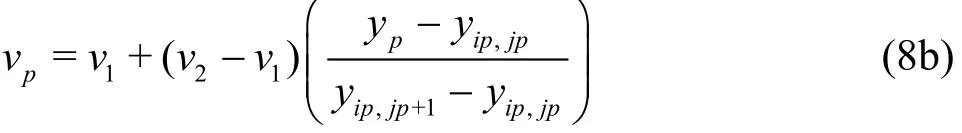
Figure 1 shows stroboscopic maps obtained analytically by Aref[2]as superimposed snapshots of the particle positions taken exactly one cycle apart for different values of μ for times up to 500T. For μ=0.05, the motion of the particles is generally periodic and observes closed orbits. For μ≥0.10,chaotic regions develop close to the blinking vortices.As μ increases further, the chaotic region grows until it fills much of the computational domain. Figure 2 reveals the corresponding stroboscopic maps obtained using the present Lagrangian particletracking model with values of flow velocity determined by interpolation. The results are in reasonable qualitative agreement with those obtained by Aref[2],indicating that the interpolation scheme is working satisfactorily. Next, the particle positions are considered after different numbers of blinking vortex cycles where an initial square array of 6 400 particles is divided into four quadrants, each of different colours forμ=1.00. The Lagrangian particle-tracking results in Fig. 3 show that mixing is more rapid and widespread when a higher value of μ is considered.Transition to chaos is evident in regions near the stirrers, with whorls and tendrils evident at the periphery.

Fig. 3 (Color online) Numerically predicted particle positions in the bilinear interpolated flow field induced by a pair of blinking vortices when μ=1.00

4. Advection of particles in the vicinity of a groyne

4.1 Particle advection in a pair of adjacent side-wall cavities

We now consider the flow past a side-wall expansion containing an idealized groyne in a rectangular open channel, following previous laboratory measurements by Tuna and Rockwell[14]who examined self-sustained resonant oscillations due to phase shifts in standing wave modes in the cavities and undulations in the separated shear later, in flow past a pair of adjacent side-wall cavities. The shallow flow solver is used to reproduce the flow conditions in a qualitatively similar configuration to that considered by Tuna and Rockwell. In our cases, the main channel is 700 mm long and 475 mm wide, with flow entering from the left hand end of the open channel. After an initial reach of 200 mm, the channel widens abruptly into a side-wall expansion of length 300 mm and additional width 225 mm. The expansion zone contains a groyne of 10 mm width that projects outward 225 mm, perpendicular to the channel wall. The groyne effectively divides the region of the side-wall expansion into a pair of adjacent side-wall cavities.After the side-wall expansion region, the channel again abruptly becomes 475 mm wide. The mean water depth is 38 mm. We consider two cases, where the inlet velocity, UI, is set to 273 mm/s and 475 mm/s,respectively.

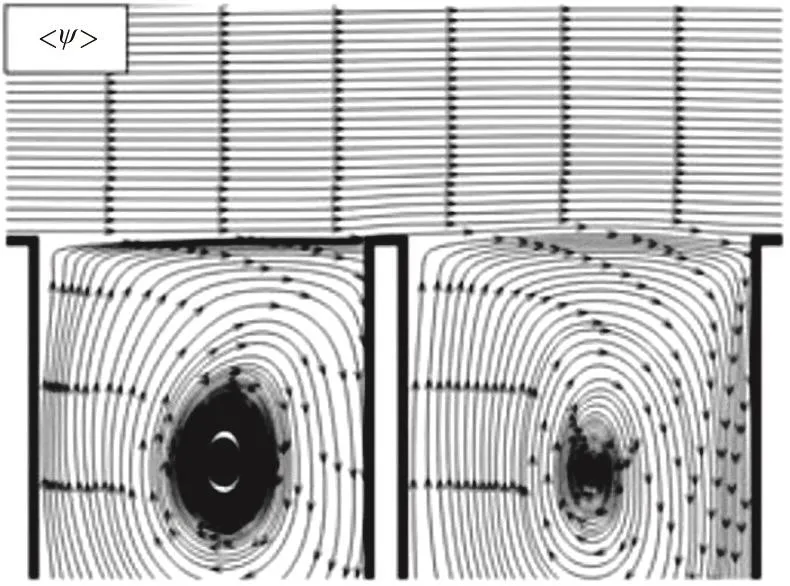
Fig. 4 Time-averaged stream function contours during a transverse mode of a gravity standing wave in a pair of adjacent side-wall cavities in open channel flow obtained from PIV measurements by Tuna and Rockwell[14]

Figure 4 shows a typical set of stream function contours obtained by Tuna and Rockwell from time-averaged PIV velocity measurements for flow past a pair of adjacent side-wall cavities. In the present work, the numerical model is based on a uniform 280 by 280 grid that covers an overall computational domain, measuring 700 mm by 700 mm,which includes the open channel and side-wall cavities. For UI=273mm/s , the eddy viscosity is set to 9.992 mm2/s, and the time step Δt=0.01s. For UI=475mm/sthe eddy viscosity is 17.264 mm2/s,and the time step Δt=0.001s. In both cases, the overall simulation time is 20 s. It should be noted that,after grid convergence was checked, the time step was selected so that the Courant number remained below unity. Figure 5 displays the steady state stream function contour results for the two cases considered using the present shallow flow solver. The contours indicate that larger vortices are produced in the two side-wall cavities at the higher value of inlet velocity,as would be expected. The present results are in qualitative agreement with those of Tuna and Rockwell[14](Fig. 5), implying that the shallow flow solver gives a potentially useful representation of flow-induced vortices in adjacent side-wall cavities separated by a single groyne.

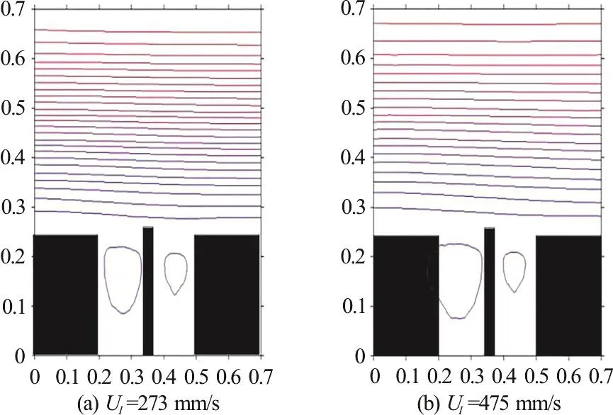
Fig. 5 (Color online) Stream function contours for open channel flow past a pair of adjacent side-wall cavities

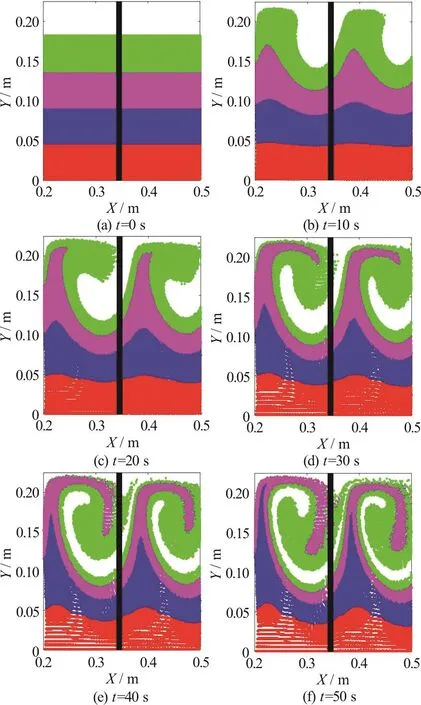
Fig. 6 (Color online) Particle advection in a pair of adjacent side-wall cavities for UI =273mm/s with time

The coupled shallow flow and particle-tracking model is then used to simulate advection and mixing processes in the side-wall cavities divided by the groyne, owing to the presence of the two recirculation zones, one in each cavity. To visualize particle mixing,the space within each cavity is filled with four layers of particles, the layers containing red, blue, purple and green particles, respectively. In this study, 54 000 particles are released, uniformly distributed throughout the cavities. Here, the time step used by the Lagrangian particle tracker is 0.5 s. Figure 6 shows snapshots of the particle positions at different times after their release, for a case where the inlet velocity is 273 mm/s. At first, the northern green and purple layers undulate. The undulations then develop standing waveforms which then curl over and form whorls. The blue layer gradually gets pulled towards the main stream, and exhibits cuspate peaks.

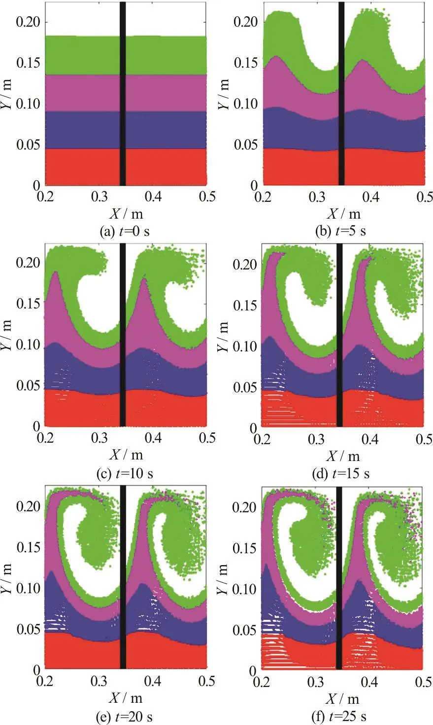
Fig. 7 (Color online) Particle advection in a pair of adjacent side-wall cavities for UI =475 mm/s with time

As can be seen in Fig.7, similar results are obtained for the higher inlet velocity of 475 mm/s,though the roll up of the magenta and green layers takes place more quickly.

Fig. 8 (Color online) Mixing of an array of 8 000 particles in an open rectangular channel containing two groynes

4.2 Mixing of particles in a rectangular channel containing a pair of parallel groynes

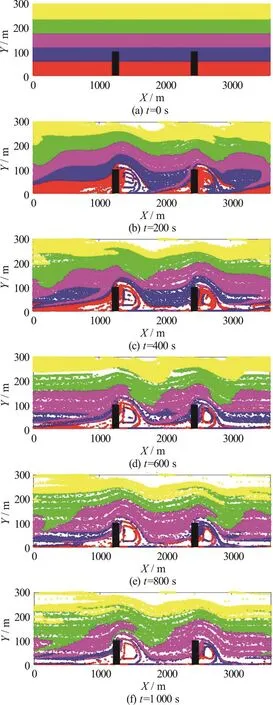
Fig. 9 (Color online) Mixing of an array of 54 000 particles in an open rectangular channel containing two groynes at different times

The coupled shallow water and particle-tracking model is now used to simulate particle advection in a rectangular open channel containing a pair of groynes.Here, the channel has plan dimensions of 3 600 m×300 m. The inlet velocity is 0.5 m/s, Reynolds number is 100, water depth is 1 m, and eddy viscosity is 0.5 m2/s.The time step is 5 s, satisfying the Courant criterion,and the simulation time to flow steady state is 4 000 s.To study particle mixing in the vicinity of the groynes,the particle-tracking model is then used to simulate trajectories of an initially rectangular array of 8 000 particles, with five colour bands, which is released upstream of the first groyne. Figure 8 shows the advected distributions of the particles at intervals of 200 s after the initial release into the steady state flow.It can be seen that the red particles become stretched along a tendril, with blue, magenta, green, and yellow particles becoming more spread out as time progresses from t=0 s (the time of particle release) to t=1000 s. Figure 9 shows the results obtained in the same rectangular channel containing two groynes, this time with an array of 54000 particles that initially entirely fill the domain, the snapshots indicate the evolving particle distributions obtained with time.Here, the yellow particles become the most separated over the long term, being advected by the main current in the channel. The red particles are initially the least separated because many become temporarily trapped in the recirculation zones.

5. Conclusions

A coupled shallow water solver and Lagrangian particle-tracking scheme has been constructed using 2ndorder finite differences in space and 4thorder Runge-Kutta integration in time. The particle-tracking algorithm was verified for periodic and chaotic advection in the alternating flow field of a pair of blinking vortices. Close agreement was obtained with analytical results presented in the literature by Aref[2],it should be noted that the present particle tracking model used an interpolated discretized velocity field instead of the continuous analytical velocity field. As the stirrer strength μ increased from 0.05 to 1.50,the chaotic region grew until it filled much of the computational domain, in accordance with Arefʼs findings. The coupled shallow water flow and Lagrangian particle-tracking model was further validated against laboratory data for open channel flow past a pair of adjacent side-wall cavities obtained by Tuna and Rockwell[14]. Results were presented for the advection of different coloured tracer particles in the region of the side-wall cavities and it was found that the majority of particles remained trapped in the side-wall cavities, with a tendency for the particles to roll up into a single whorl that filled each cavity.Mixing of particles in a rectangular channel containing a pair of parallel groynes, oriented perpendicular to the lateral walls, has also been simulated using the coupled shallow flow and particle-tracking model.The use of different colour bands of particles highlighted particle trapping that occurred immediately downstream of each groyne within the recirculation zones, with the majority of particles passing the ends of the groynes (in the main through-flow stream).

Acknowledgement

The first author is grateful to the University of Edinburgh which partly funded this research.