Yu-Hsiang Chen, Keh-Han Wang

Department of Civil and Environmental Engineering, University of Houston, Houston, USA

Abstract: This paper presents a newly developed 3-D fully nonlinear wave model in a transient curvilinear coordinate system to simulate propagation of nonlinear waves and their interactions with curved boundaries and cylindrical structures. A mixed explicit and implicit finite difference scheme was utilized to solve the transformed governing equation and boundary conditions in grid systems fitting closely to the irregular boundaries and the time varying free surface. The model’s performance was firstly tested by simulating a solitary wave propagating in a curved channel. This three-dimensional solver, after comparing the results with those obtained from the generalized Boussinesq (gB) model, is demonstrated to be able to produce stable and reliable predictions on the variations of nonlinear waves propagating in a channel with irregular boundary. The results for modeling a solitary wave encountering a vertical cylinder are also presented. It is found the computed wave elevations and hydrodynamic forces agree reasonably well with the experimental measurements and other numerical results.

Key words: Solitary wave, curvilinear coordinate transformation, curved channel, wave scattering, hydrodynamic forces

Introduction

Accurately modeling wave transformation induced by the structure or irregular boundaries is practically important to coastal and offshore engineering applications. Over the past decades, the interactions between water waves and cylindrical structures have been investigated. Isaacson[1]derived the analytical solutions on wave force and free-surface run-up for a solitary wave encountering a vertical cylinder.Higher-order solutions for the diffraction of a solitary wave around a vertical cylinder were obtained by Basmat and Ziegler[2]. For numerical solutions,Boussinesq equations are commonly used to model the interaction between nonlinear shallow water waves and structures. Wu[3]developed a generalized Boussinesq (gB) two-equation model for modeling a 3-D nonlinear wave propagating in shallow water based on the concept of layer-mean velocity potentials.For the study of fully nonlinear long waves, Wu[4]further derived the fully nonlinear and weakly dispersive Boussinesq equations. Using the finite difference method, Wang et al.[5]numerically solved the gB equations to investigate the scattering of a solitary wave by a bottom-mounted vertical cylinder.Later, the concept of multiple grid systems was utilized to model the interaction between solitary waves and arrays of cylinders[6-7].

The finite element method was also introduced into the numerical approach of solving the Boussinesq equations where it had the advantage of using non-uniform or unstructured grids, but raised with concerns of long simulation time. Ambrosi and Quartapelle[8]and Woo and Liu[9]investigated the propagation of solitary waves by means of their respective finite element based Boussinesq models.Recently, Zhong and Wang[10]developed a timeaccurate stabilized finite element model to study the diffraction processes of waves of two classes, namely weakly-nonlinear-and-weakly-dispersive and fullynonlinear-and-weakly-dispersive waves, encountering cylindrical structures.

Fully 3-D models can provide more detailed information on wave motion, velocity distribution,and especially the 3-D wave loads on structures. Yang and Ertekin[11]applied the boundary element method to calculate the solitary wave induced forces on a vertical cylinder. Ma et al.[12]and Kim et al.[13]simulated the interactions between a vertical cylinder and steep waves by using a 3-D finite element model.Later, Eatock Taylor et al.[14]combined the boundary element and finite element methods to perform numerical wave tank simulation. Appling an efficient non-hydrostatic finite volume model, Ai and Jin[15]performed numerical simulations of solitary waves interacting with a vertical cylinder, an array of four cylinders, and a submerged structure. Choi et al.[16]solved the 3-D Navier-Stokes equations by means of a finite difference method to model the run-up of a cnoidal wave around a bottom mounted cylinder.Experimentally, Yates and Wang[17]carried out a series of experimental measurements of free-surface elevations around a vertical cylinder and induced forces for the case of a solitary wave scattered by a vertical cylinder.

For 3-D computation, the finite difference method is an effective numerical scheme to solve the model equations. To extend the application of the finite difference method to simulate wave transformation induced by irregular boundaries, coordinate transformation technique, though limited to 2-D domain, has been utilized in various cases of non-orthogonal boundaries such as breakwaters,cylindrical structures, shorelines, or channels[6-7,18].For nonlinear wave modeling, Boussinesq’s equations with coordinate transformations can provide solutions to describe nonlinear long waves propagating in variable topographies. Shi and Teng[19]and Shi et al.[20]adopted the curvilinear-coordinate based gB models to investigate wave evolutions for a solitary wave propagating through a significantly curved water channel. Higher-order Boussinesq’s equations were applied in a curvilinear coordinate system to simulate waves propagating through curved channels[21-23].Additionally, the boundary-fitted coordinate transformations were combined with the solvers of the Navier-Stokes equations to investigate nonlinear waves traveling in a curved channel[16,24]. Different from using the curvilinear coordinate transformation approach, Nachbin and Da Silva Simões[25]adopted the Schwarz-Christoffel transformation into the gB equations to study the interaction of a solitary wave with a sharp-cornered and a smoothly curved 90°bend.

For wave modeling, if the focus of the study is to determine the free-surface elevations and vertically averaged flow variables, then the vertical-averaged or vertically-integrated models, such as the Boussinesq models described in literatures, may be applied to obtain the limited wave solutions. However, the detailed 3-D variables, such as the velocity and pressure distributions, especially showing the variations along the vertical direction, will be missed from using the Boussinesq models (e.g., gB model).Additionally, when modeling wave and structure interactions, the Boussinesq models are limited only to the cases with structures that are extended from domain bottom to the free-surface and cannot handle the conditions with either floating or completely submerged structures. The simulations of wave interactions with either partially submerged or fully immersed bodies, due to the existence of additional inner domains either beneath or above the structures,can only be modeled by a complete 3-D model as presented here.

With the purpose of wider applications on modeling wave propagation and wave-structure interactions,this study is to develop a 3-D fully nonlinear wave model by solving the 3-D Laplace equation and specified boundary conditions on the free surface and structural surface to investigate the interaction process between solitary waves and cylindrical structures. In order to have the computational grids fit closely to the irregular structural boundaries and to trace the time-varying free surface for the numerical advantage,a transient 3-D curvilinear coordinate transformation technique is adopted to develop a new set of curvilinear-coordinate based model equations. Numerically the multiple grid systems with curvilinear grid points covering the regions close to the structures separating from those regular grids for regions far outside of the structures are used. For the verification of the developed model, results considering the cases of solitary waves and their interactions with a curved channel and with a bottom mounted and surfacepiercing cylindrical structure are compared with measured data and other published numerical solutions.

1. Mathematical formulations

1.1 Governing equations

For the convenience of model development and results presentation, all physical variables are nondimensionalized according to,andrespectively as the length, time, and velocity scales. A variable with superscript “*” represents the dimensional form of that variable. The Cartesian coordinates were chosen as the original coordinate system to formulate the governing equation and the boundary conditions. The x- and y-axes represent the two horizontal coordinates while z-axis points upward with z=0 being set at the level of the undisturbed free surface. z=ζ(x, y, t) denotes the displacement of the free surface from the undisturbed water level and t is time. The bottom of flow domain is horizontal and is placed at z*=-or in dimensionless form z=-1, whereis a constant water depth. It is assumed that the fluid is incompressible and inviscid and the motion irrotational. The velocity potential φ of the wave motion satisfies the Laplace equation, which is described in dimensionless form as

1.2 Boundary conditions

The kinematic free-surface boundary condition(KFSBC) can be written as

The velocity components u, v and w can be related to the velocity potential as u= ∂φ/∂x, v=∂φ /∂y and w= ∂φ/∂z, respectively. While the dynamic free-surface boundary condition (DFSBC) is given as

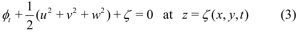
where the subscripts denote the partial derivatives.

For modeling the interactions between nonlinear waves and cylindrical structures in a domain of wave channel with two side walls, the boundary conditions on the rigid side walls and the circular cylinder surface follow that the normal fluid velocity vanishes there. We have

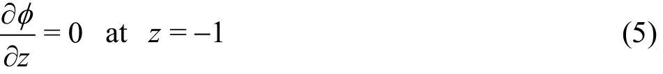
where n is the unit normal direction to a solid boundary surface. In addition, no fluid penetrating at the flat solid bottom boundary leads to the following b ottom boundary condition

The open boundary conditions control the waves propagating out of the computational domain without the adverse impact from wave reflection. Following Chang and Wang[26], the extended open boundary conditions are given as

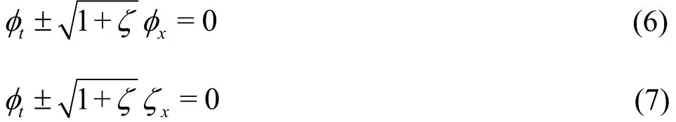
where the + or - sign is referenced according to the downstream or upstream boundary.

1.3 Initial condition for incident solitary waves

To introduce an initial 3-D velocity potential of an incident solitary wave, the relationship between the original velocity potential φ(x, y, z, t) and the layermean velocity potential(x, y, t), where=, as given in Wang et al.[5]

is utilized. According to Schember[27]and Wang et al.[5]

where

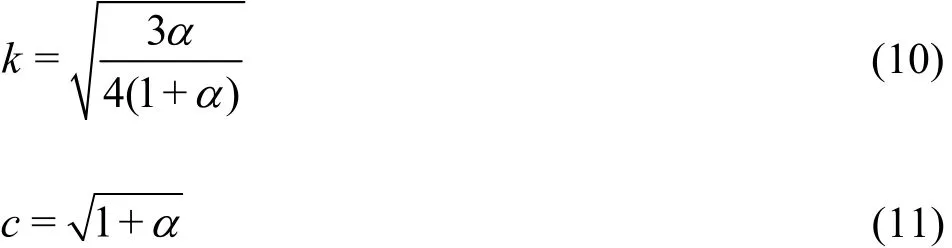
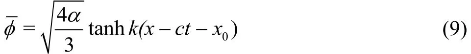
and α is the dimensionless wave amplitude. The corresponding free surface elevation is expressed as

The 3-D velocity potential for an incident solitary wave can be derived by substitutingfrom Eq. (9)into Eq. (8) to have

Equation (12) can be used as an initial wave condition by setting t=0 and letting the peak of a specified solitary wave be situated at x=x0. For modeling wave and cylinder interaction, the initial wave peak location is selected to be sufficiently far away from the cylinder as suggested by Wang et al.[5].

1.4 Forces on a cylinder

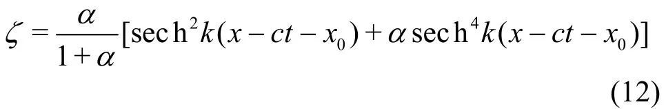
The wave-induced hydrodynamic force F acting on a bottom mounted vertical cylinder can be calculated by integrating the pressure on the cylinder surface, where the pressure, p, is computed from the Bernoulli equation

For the convenience of force comparisons with other published results for the cases of a bottom mounted and surface piercing cylinder, the inline force coefficient CfH(t) (as normalized by)is defined as the integral of the x-component of the excess pressure (p+z) over the surface of the cylinder in contact with the fluid. The form of the force coefficient is

where R is the radius of a cylinder considered in the study and θ is the angle of angular direction measured from the negative x-axis.

2. Numerical method

2.1 3-D transient curvilinear coordinate transformation

In this study, a 3-D transient curvilinear coordinate transformation technique is utilized to transform the transient grid points in Cartesian coordinates(x, y, z; t) into transient curvilinear coordinates (,ξ η, γ; τ) for multi-grid modeling application. The transient effect on the computational grids is limited to the vertical coordinate. This indicates that the physical z-coordinates vary at each time level according to the updated vertical domain at a given location. The transformation of the governing equations and the boundary conditions into the transient curvilinear coordinate system is summarized in the following.

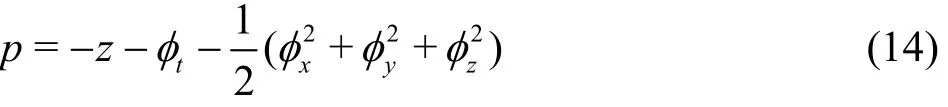
Using the 3-D velocity components, u, v and w and their corresponding expressions in the curvilinear coordinate system

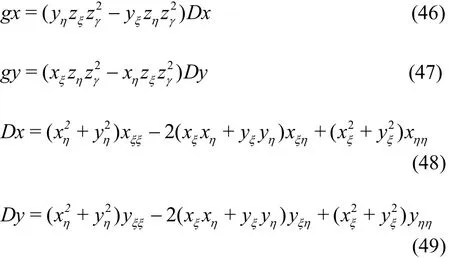
the Laplace equation (Eq. (1)) in Cartesian coordinates can be transformed as

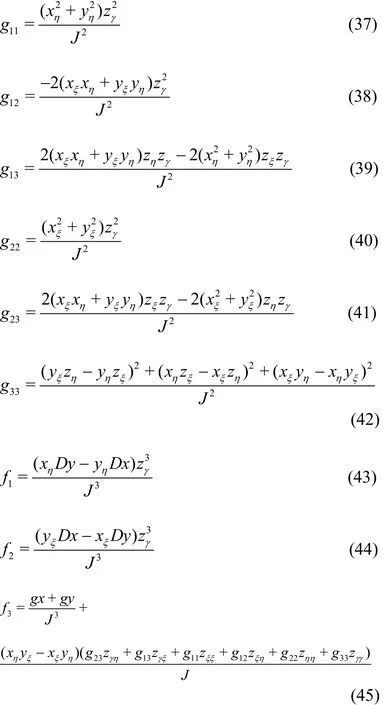
where the subscripts of the velocity potential denote the partial derivatives and the formulations of g11,g12, g13, g22, g23, g33, f1, f2and f3are given in Appendix A.

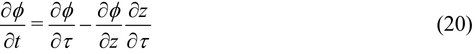
For the time derivative of the velocity potential,we have

The free-surface boundary conditions described in Eqs. (2), (3) are transformed as

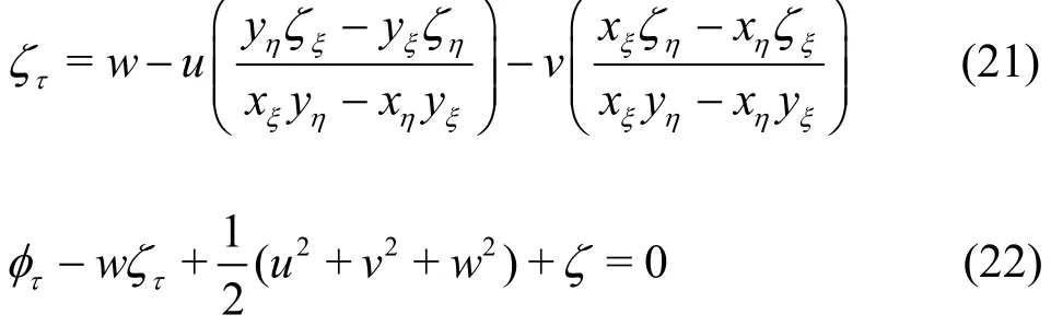
where u, v and w are 3-D velocity components given in Eqs. (16)-(18) respectively. Similarly, the open boundary conditions as given in Eqs. (6), (7) are reformulated in the transformed coordinate system to have

2.2 Numerical approach and formulations

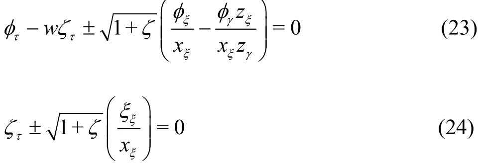
The finite difference method is applied to solve the governing equation and boundary conditions.Following the usual notations,andare defined as=φ(iΔξ,jΔη,kΔγ,nΔ t ) and=φ( iΔξ,jΔη,nΔ t), in which i,j and k are grid indices along respectively ξ, η and γ directions,n is the time level index, Δt is the time step, and Δξ=Δη=Δγ=1 are spatial mesh sizes in ξ, η and γ directions. The central difference scheme when applied to discretize the spatial derivatives in the governing equation (Eq. (19)) yields

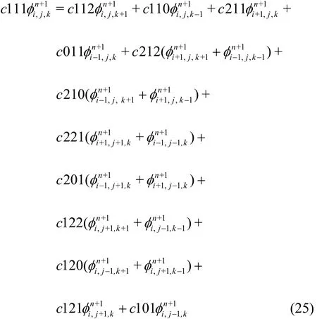
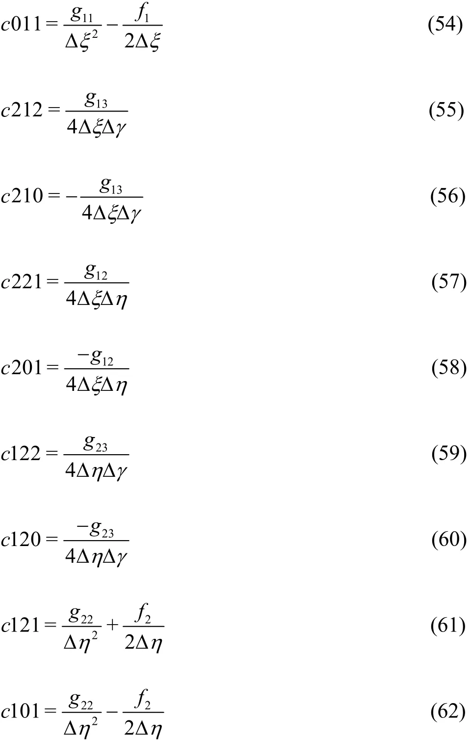
where the expressions of coefficients c111, c112,c110, c221, c011, c212, c210, c221, c201,c122, c120, c121 and c101 are summarized in Appendix B.

where

and

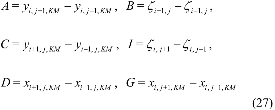
in which

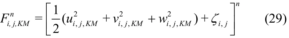
In Eqs. (26)-(29), the terms with superscript n ordenote respectively the values at the n time level or the provisional values attime level through explicit computation. The index KM represents the vertical grid points at the water surface layer. Through the iteration procedure, the updated values ofandare calculated from the following implicit finite difference formulations

in which

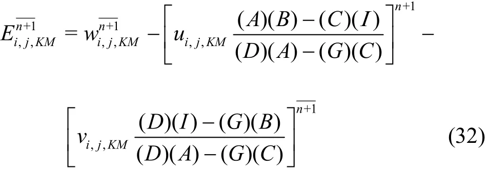
and

The averaging procedures using values obtained from the explicit and implicit computations forandin kinematic free-surface boundary condition and forandin dynamic free-surface boundary condition are applied to further the determination of the final values of the free surface elevationand velocity potentialat(n+1)Δt time. The described formulations are shown below

2.3 Multiple-block computations

For modeling a solitary wave interacting with a fixed cylindrical structure, a single set of curvilinear grids can generally represent well the flow domain.However, the concern is that potentially the numerical instability and singularity may appear when applying the structural boundary conditions on the grid points located around the cylinder surface and the cuts of the grid system, especially at points in front of the structures that receive the direct impact from the incident nonlinear waves. In order to avoid the numerical errors caused by inappropriate grid points within a single set of curvilinear grid system, a multi-grid system and a multiple-block computational method as introduced by Wang and Jiang[6]is adopted for the present study. Polar grids (inner grids) are introduced to cover the region close to and on the cylinder surface while the rectangular grids (outer grids) are extended over the remaining fluid domain outside of the cylinder. Overlapped grids between the inner and outer grid systems are arranged to allow the interpolation of physical variables at the grid interfaces for the numerical iteration and check of solution convergence. Figure 1 shows the distribution of the inner polar grids and part of the outer rectangular grids with the thick black line representing the inner boundary of the rectangular grids.

After an initial solitary wave introduced in the entire computational domain, to proceed to the next(or new) time level, the numerical procedure for the multi-grid systems is to firstly compute the velocity potentials and wave elevations throughout the outer rectangular grids. Then, a three-point interpolation scheme using the solutions of neighboring rectangular grids is carried out to provide the values of φ and ζat the grid points of the outer boundary of the inner polar grids. With the boundary values are determined,the computation moves to the inner polar grids. Once the values of physical variables within the inner polar grids are calculated, the velocity potentials and wave elevations of the inner boundary of the outer rectangular grids are updated by the three-point interpolation scheme using the values obtained from the computation within the inner polar grids. The procedures are repeated until the converged solutions are obtained at the new time level. The computation continues until the allotted final time level.

Fig. 1 (Color online) Two-grid system with arranged grid points for a bottom mounted and surface piercing cylinder situated in a computational domain

For the vertical direction (z-direction), the zcoordinates are calculated using the algebraic grid generation method as

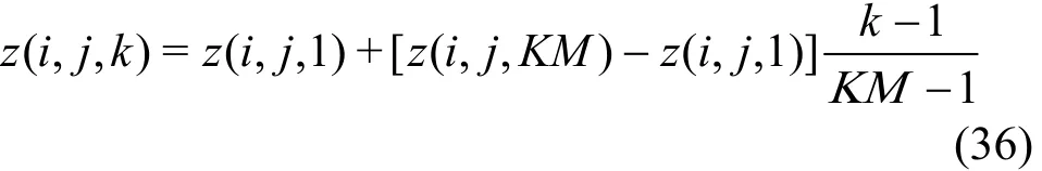
Again, KM represents the maximum index of the grid points along the z-direction and z( i, j, KM)denotes the vertical coordinate of the free surface. An example plot of the grid system along the x- z plane is presented in Fig. 2.

3. Model applications-results and discussions

3.1 Solitary waves propagating in a curved channel

Before the application of the present model to simulate wave propagation in a curved channel, a simple case considering a plane solitary wave propagating in a straight rectangular wave channel was performed to test model’s stability and accuracy. The computational domain described in dimensionless form is 0≤x≤80 and 0≤y≤3. Vertically,KM=21. The amplitude of incident solitary wave α is set to be equal to 0.4. A sequence of time series plots of the free-surface elevations along the central plane of the numerical channel are presented in Fig. 3.The results shown in Fig. 3 suggest that the present numerical model can produce a stable wave profile representing the propagation of an incident solitary wave over a considerable distance. Throughout the process of wave propagation, the wave amplitude remains as a constant value of 0.4. As a result, the model is demonstrated to be able to produce consistent and accuract solutions describing propagation of solitary waves.

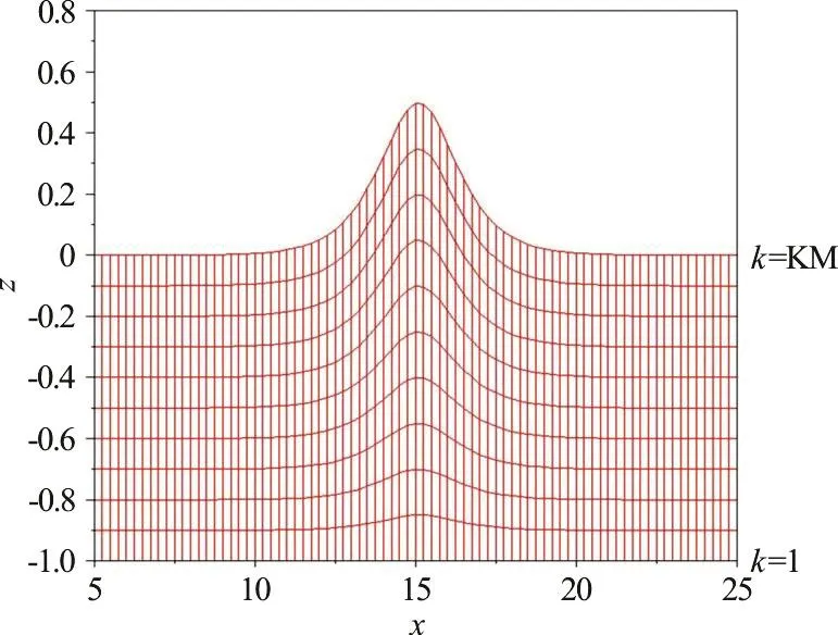
Fig. 2 (Color online) An x-z plane view of the grid system in the physical domain

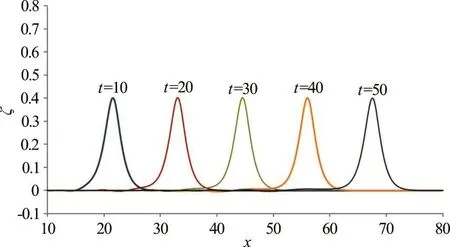
Fig. 3 (Color online) A sequence of time series plots of numerically generated solitary waves propagating in a channel of constant depth (α=0.40)

As an extension to test the capability of modeling waves in a channel of arbitrary shapes, the application of the present nonlinear wave model in simulating a solitary wave propagating through a 180° curved (U-shaped) channel was performed. The dimensionless width of the channel is 12.5 whereas the length along the central plane is 95. The radii of the inner wall and the outer wall of the channel at the curved section are 5 and 17.5, respectively. The amplitude of an initial plane solitary wave is set as 0.3. In order to verify the present 3-D fully nonlinear solutions, the gB twoequation model established by Wang et al.[5]is also applied to calculate the wave elevations along the curved channel for comparisons. Computed wave elevations at three positions along each of three selected cross sections (A-C) throughout the channel are compared. The locations of three cross sections are shown in Fig. 4. Along each cross sections, three chosen positions with each marked by a red dot are denoted by “inner wall”, “center of channel”, and“outer wall”, respectively.

Fig. 4 (Color online) The location comparisons of time variation of freesurface elevation

The comparisons of time varying free surface elevations obtained from the present model and from the gB two-equation model at each identified location are presented in Figs. 5-7. Figure 5 illustrates the comparisons of time varying free-surface elevations obtained from gB model and the present 3-D fully nonlinear model at the position of “outer wall” in cross section A. As there is a nonlinearity difference of the two models where one is the weakly nonlinear and weakly dispersive based gB model and the other is the present fully nonlinear based model, an insignificant dimensionless phase shift of 0.8 is noticed. Without considering the phase shift, the results in Fig. 5 suggest that both models predict nearly identical wave variations including wave peak throughout the entire wave transformation process in the curved channel. It is noticed in Fig. 5 that when the solitary wave propagates into the curved section and encounters the outer wall of the channel, the waves piles up in front of the outer wall and follows with wave reflection. Two wave peaks that occurred at the channel center are noticeable in Fig. 6. Moreover,due to the continuing process of wave diffraction and reflection between the inner and outer walls, the occurrence of crossed wave oscillation generates varying wave peaks across the channel (Fig. 7). Again,from the results presented in Figs. 6, 7, the gB and present nonlinear wave models obtain consistent and agreeable wave profiles. This comparison study confirms that the present 3-D fully nonlinear wave model can provide stable and accurate predictions on wave propagation and transformation in a domain with complex geometry. Additionally, the conservations of mass and energy have also been verified.

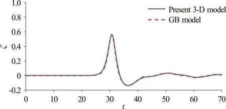
Fig. 5 (Color online) Comparisons of time variations of freesurface elevations obtained from gB model and the present 3-D fully nonlinear model at a representative position of “outer wall” along cross section A (initial wave amplitude α=0.30)

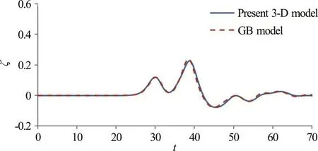
Fig. 6 (Color online) Comparisons of time variations of freesurface elevations obtained from gB model and the present 3-D fully nonlinear model at a representative position of “center of channel” along cross section B (initial wave amplitude α=0.30)

Fig. 7 (Color online) Comparisons of time variations of freesurface elevations obtained from gB model and the present 3-D fully nonlinear model at a representative position of “inner wall” along cross section C (initial wave amplitude α=0.30)

As discussed above when using initial wave amplitude of 0.3, agreeable wave elevations obtained either from gB or present nonlinear model are concluded according to the results presented in Figs.5-7. It would be interested in examining the effect of higher nonlinearity on the wave transformation and the comparisons between gB and present model results for the case of a solitary wave propagating through the curved channel. An initial wave amplitude of α=0.52 was selected for the simulation. The time varying wave profiles from the gB and present nonlinear models at the region with a stronger interaction (along section A, for example, at the location of “outer wall”) are presented and compared in Fig. 8. In general, the computed wave elevation patterns from either the gB or present model are still very similar. It is noticeable, at the location of “outer wall” that is subject to the direct wave impact from a higher initial wave amplitude (such as α=0.52), the present nonlinear model predicts higher wave peak than that from the gB model.

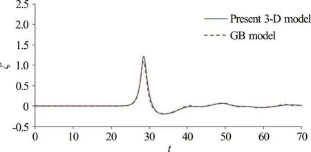
Fig. 8 (Color online) Comparisons of time variations of freesurface elevations obtained from gB model and the present 3-D fully nonlinear model at a representative position of “outer wall” along cross section A (initial wave amplitude α=0.52)

A series of contour plots of the free-surface elevation for a solitary wave of α=0.30 propagating through a 180° curved channel are presented in Fig. 9. The solid and dash lines in the contour plots represent respectively the positive and negative values of the wave elevations. From Fig. 9, it is noted that the solitary wave maintains as a uniform wave profile before it enters the curved portion of the channel at t=15. As the solitary wave propagates into the curved channel at t=25, the nonuniform distribution of the wave peak across the channel starts to form.Owing to the centrifugal effect, the wave elevation with the highest amplitude near the outer wall shows the decreasing trend towards the inner wall of the channel. The wave encountering process on the outer wall and its water surface can reach up to about 0.45 at t=35. Due to the length difference between the inner an d t he ou ter wall s of th e bended p art of thecurved wave front can be noticed,a curved wave front can be noticed. At t=45, during the process of main wave propagating towards the downstream portion of the curved channel, due to the effect of wave reflection, the high peak of the wave is observed to move to the center of the channel.Following the above described wave transition, the main wave close to the outer wall encounters the wall again and results in the increase of the free-surface elevation of the main wave near the outer wall at t=55. Two high wave peaks coexist along the main wave crest. From t=55 to t=65, the position of the peak of wave elevation near the outer wave gradually catches up with the peak of the leading wave near the inner wall. It can be seen the transmitted waves are not recovered as the shape of the original incoming solitary wave.

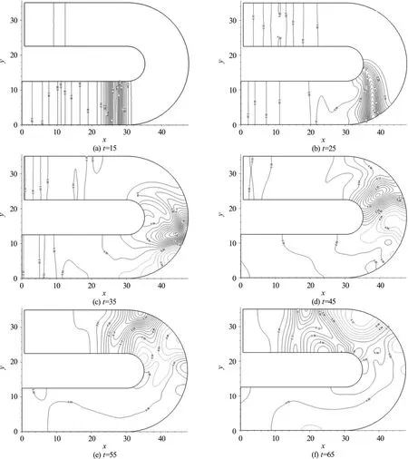
Fig. 9 Contour plots of free-surface elevation ζ for α=0.30 at different time steps

3.2 Solitary waves interacting with a bottom mounted and surface piercing vertical cylinder

The developed model is also applied to simulate a solitary wave interacting with a vertical surfacepiercing cylindrical structure. The fluid domain with a vertical circular cylinder for this study is shown in Fig.10. The dimensionless radius of the cylinder (R) is 1.59 and the cylinder is fixed at the center of the channel. The amplitude of the incident solitary wave is given as α==0.4. The values of the radius of the cylinder and the amplitude of the solitary wave were selected to be the same as those used in the experimental studies conducted by Yates and Wang[17]for the purpose of comparing the present numerical results to the experimental measurements. The phy-sical domain is 0≤x≤80 and 0≤y≤35. Locally refined grids are arranged to cover the areas close to the cylinder and Δt=0.1 (see Fig. 10).

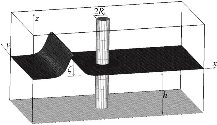
Fig. 10 Coordinate system for the description of the governing equations

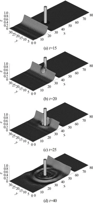
Fig. 11 Three-dimensional perspective view plots of free-surface elevation ζ for α=0.40 at selected instants of time

Figure 11 presents a time sequence of 3-D perspective view plots of the free-surface elevation showing the process of a solitary wave interacting with a cylinder. At t=10, a simulated stable solitary wave as the incident wave can be noticed to propagate towards the bottom mounted vertical cylinder. While the peak of the solitary wave impacts on the cylinder at t=20, the solitary wave piles up to a maximum value of the free-surface elevation in front of the cylinder surface. After the primary wave propagates past the cylinder, as shown at t=25, the backscattering and forward-scattering waves are formed around the cylinder. Additionally, as part of the waves is emerged as the back-scattered waves after wavecylinder interaction, the wave height of the central part of the primary waves is lower than the other parts of the primary waves. However, those wave portions can still keep the same propagating speed as other primary waves. While the solitary wave propagates over 20 water depths beyond the cylinder at t=40, a group of scattered waves travel further away from the cylinder and expand over the upstream and downstream regions of the cylinder. Moreover, the central part of the primary wave transitions back to nearly its original amplitude and as a whole the wave recovers as a solitary wave propagating towards downstream.

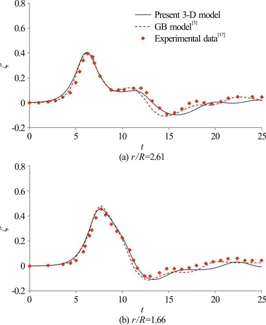
Fig. 12 (Color online) Comparisons of time variation of freesurface elevation along θ=0° obtained from the present 3-D nonlinear model, the gB model[5] and experimental data[17]

Figures 12-16 illustrate the wave elevations in time series at selected radial locations along θ=0°,60°, 100°, 150° and 180° directions, where θ=0°points towards upstream (-x) direction and θ=180° is along the downstream direction behind the cylinder. The experimental measurements[17]and gB model results are also presented for comparisons. In Fig. 12(a), the wave elevations at θ=0° and r/ R=2.61 show the propagation of an α=0.4 solitary wave, an induced reflected wave, and a train of small oscillatory waves after encountering the cylinder. At a position close to the cylinder surface (r/ R=1.66),Fig. 12(b) reveals that the amplitude of the solitary wave increases in front of the cylinder and is followed by a negative wave propagating radially outward from the cylinder surface. Similar variation trends of the free-surface elevations at the locations of r/ R=1.35 along θ=60° direction can be found in Fig. 13. The comparisons shown in Figs. 12, 13 indicate that the present model results agree reasonably well with the experimental data and those from the gB model.

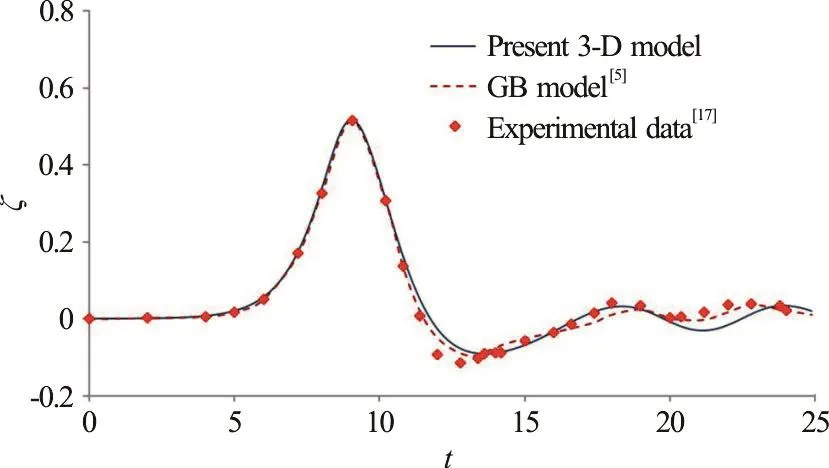
Fig. 13 (Color online) Comparisons of time variation of free-surface elevation along θ=60° at a representative position ofr/ R=1.35 obtainedfrom the present 3Dnonlinearmodel, the gB model[5]andexperimental data[17]

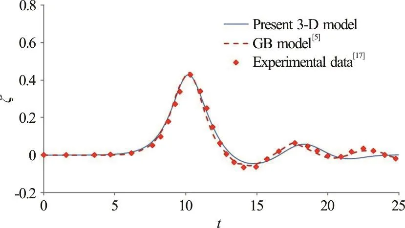
Fig. 14 (Color online) Comparisons of time variation of free-surface elevation along θ=100° at a representative position of r/ R=2.29 obtained from the present 3-D nonlinear model, the gB model[5] and experimental data[17]

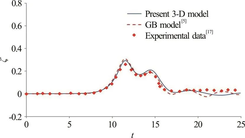
Fig. 15 (Color online) Comparisons of time variation of free-surface elevation along θ=150° at a representative position of r/ R=1.35 obtained from the present 3-D nonlinear model, the gB model[5] and experimental data[17]

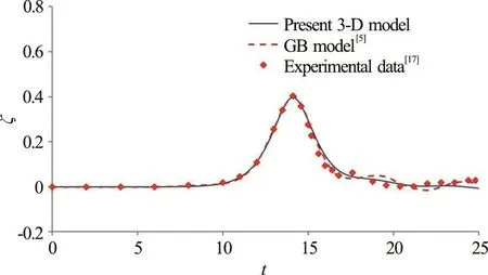
Fig. 16 (Color online) Comparisons of time variation of free-surface elevation along θ=180° at a representative position of r/ R=2.92 obtained from the present 3-D nonlinear model, the gB model[5] and experimental data[17]

Figures 14-16 illustrate the comparisons between the computed and measured free-surface profiles on the rear side of the cylinder. The wave profiles include a main solitary wave followed with a group of forward-scattered waves. Figure 14 shows the variations of the free surface along the radial direction of θ=100°. The present model predictions again match well with measured data at the location of r/ R=2.92.For the locati ons al on g θ =60°, θ=10 0° , the gB model resultsseemtofitslightlybetterthanthose from the present 3-D model. The similar variations and agreement with measurements in terms of the predicted wave profiles can also be found along the directions of θ=150° (Fig. 15). The present model can provide good predictions on the wave elevations at locations behind the cylinder. Along the direction of θ=180° (Fig. 16), it is interesting to note that the present fully nonlinear model can better predict than the gB model does the general trend of wave variation and the tailing part of the main wave. Also, shown in Fig. 16, after the main wave propagates past the cylinder, the wave amplitude in the region behind the cylinder recovers to nearly the original amplitude (e.g.at r/ R=2.92). It is demonstrated from this comparison study that the present 3-D nonlinear wave model in general can make similar or better predictions (for regions behind the cylinder) on free-surface variations of a solitary wave interacting with a bottom-mounted and surface piercing cylinder when compared to the results obtained from the gB model.

From the comparison plots presented in Figs.12-16, it can be concluded that, in general, the present 3-D nonlinear wave model and gB solver perform similarly in terms of calculating the free-surface profiles after a solitary wave encountering a vertical circular cylinder. However, the present nonlinear model can provide slightly better predictions on the wave elevations in regions behind the cylinder (e.g.,θ=150°, θ=180° ). Physically, the fluids in the regions behind the cylinder experience stronger wavewave interactions during the process where the separated main waves meet at the rear part of the cylinder. Therefore, the present fully nonlinear model as reflected from the result comparisons produces better predictions than gB model on waves behind the cylinder. Actually, with a stronger wave-cylinder interaction at the location in front of the cylinder(θ=0°), the present model also provides slightly better predictions on the variation trend of the main wave.

Fig. 17 (Color online) Comparisons of vertically averaged horizontal velocity components and obta ined from the present 3-D nonlinear modelandthegBmodelat selectedtwolocations(r/ R=1.75, θ=45°)and(r/ R=1.75,θ=135°) for R=1.59 and α=0.40

The verification of the present 3-D nonlinear model has also been carried out by comparing the vertically averaged horizontal velocity componentsandwith those from the gB solver as it can only be applied to obtain the vertically averaged variables. Theandare defined respectively as

The comparison plots showing the time variations ofandobtained from the gB and present 3-D nonlinear models at selected two locations(r/ R=1.75,θ=45°) and (r/ R=1.75,θ=135°) for a solitary wave of α=0.40 interacting with a R=1.59 cylinder are presented in Fig. 17. The results shown in Fig. 17 further confirm the performance of the present 3-D nonlinear model as the values ofandcomputed are in a fairly good agreement with those from the gB solver.

The hydrodynamic forces of solitary waves acting on the cylinder can be determined by Eq. (14).The comparisons of the time varying horizontal force coefficients obtained from the present model, gB approach, and experimental measurements for different incident wave amplitudes, such as α=0.18, 0.24,0.32 and 0.40, are given in Figs. 18(a)-18(d),respectively. In Fig. 18(a), when α=0.18, the results from either the present 3-D nonlinear wave model or the gB solver are found to match closely with the measured forces. Reasonable force predictions for the case of α=0.24 can also be noticed in Fig. 18(b).As the amplitude of the incident wave increases, e.g.,α=0.32, 0.40, the results in Figs. 18(c), 18(d)indicate that both the present fully nonlinear wave model and gB solver overestimate the maximum forces. However, it should be noted that the smaller measured maximum forces may be caused by the viscous and boundary layer effects and the small gap set between the bottom of the cylinder and the channel bottom for wave force measurements. Considering the effect of relative size of a cylinder, R, on the wave forces, Fig. 19 presents the time variations of dimensionless horizontal force induced by an α=0.40 solitary wave for cases with cylinder size varied from 1-3. It can be noted that with an increase in cylinder size the positive maximum force increases. Also, for a larger cylinder (e.g., R=3), the time varying horizontal force tends to follow more on a nonlinear variation trend with a higher positive force and a less depressed negative force distribution.

In addition to the wave elevation calculations, for the case with a larger incident wave amplitude (e.g.,α=0.40), the transition process of the force variation(See Fig. 18(d)) from the positive values to the negative ones obtained by the present nonlinear model is shown to have a slightly better fit to the measu-rements than that from the gB model. The present model is again demonstrated to not only be able to provide satisfactory predictions on the wave diffraction profiles but also the hydrodynamic forces on a cylinder subject to the interaction by an incident solitary wave.

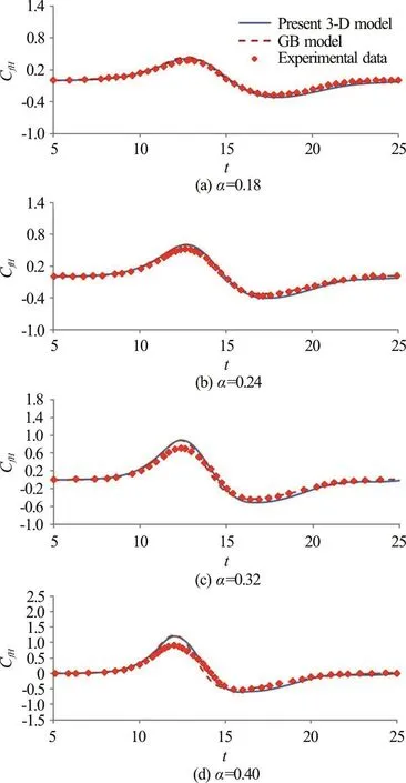
Fig. 18 (Color online) Comparisons of force coefficient CfH in time sequence

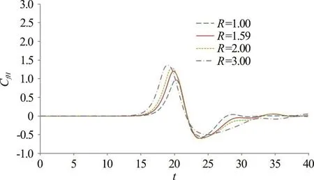
Fig. 19 (Color online) Time variations of horizontal force coefficient CfH for α=0.40 and various relative sizes in terms of dimensionless radius of a cylinder

4. Conclusion

A 3-D fully nonlinear wave model with the inclusion of the transient curvilinear coordinate transformation technique is presented in this paper. The model is firstly applied to simulate a solitary wave propagating in a 180° curved channel to demonstrate its capability of handling 3-D transient curvilinear coordinate transformation for the case of wave propagation in a domain with complex geometry.From the comparisons of the time variations of the free-surface elevations at selected locations for an up to α=0.52 incident wave, the predicted wave patterns in the curved channel obtained from the present model are shown to be similar to those calculated from the gB two-equation model. Thus, the present 3-D fully nonlinear wave model can provide stable and desired predictions on nonlinear waves propagation in a channel with irregular boundary. The present model is also extended to solve a solitary wave encountering with a bottom mounted and surface piercing vertical cylinder. During the interaction process, the solitary wave gradually piles up to a maximum value of the free-surface elevation while the main wave approaches the cylinder. After the main wave passes the cylinder, a group of outward-propagating scattered waves expands over the upstream and downstream of the cylinder. The main wave at further downstream is nearly recovered back to its original form of the incident wave. The time variations of the free-surface elevation obtained by the present model match closely with the experimental measurements.Moreover, the hydrodynamic forces calculated from the present model have reasonable agreement with the measured ones for the cases up to α=0.40 wave amplitude. In this study, the successful application of the developed 3-D fully nonlinear wave model in simulating the interaction between a solitary wave and a fixed cylindrical structure is achieved.

Appendix A

The expressions of g11, g12, g13, g22,g23, g33, f1, f2and f3in Eq. (19) are given as

Appendix B

The formulations of c111, c112, c110, c211,c011, c212, c210, c221, c201, c122, c120,c121 and c101 in Eq. (25) are