Jacob RUBINSTEIN

(Dedicated to Professor Haim Brezis on the occasion of his 70th birthday)

1 Introduction

People start losing their ability to contract the eye’s lens at about the age of 45.This leads to deteriorating near-field vision,a condition known as presbyopia.If a person suffers also from myopia or hyperopia,then that person needs vision correction both for far vision and near vision.One option is to keep two pairs of spectacles;another option is to use bifocal lenses,where a small lens for near vision is fused onto a larger lens for far vision.The bifocal solution is based on the fact that as the eye accommodates,that is,tries to view a near-by object,it also converges towards the nose.Therefore,the smaller lens in a bifocal is fused in the nasal part of the larger lens.

A major drawback of bifocals is that they create a discontinuity in the lens structure,as well as a discontinuity in its optical behavior.This implies discomfort to the wearer and also an undesired cosmetic effect.Therefore,there were many attempts to design a smooth surface that will provide slow transition from far vision to near vision.In addition to overcoming the two drawbacks of bifocals,such a smooth multifocal lens could provide good vision at all intermediate distances.

The purpose of this paper is to explain the mathematical foundations of multifocal lens design.As will be shown,a high quality design requires a variety of mathematical tools,including PDEs,numerical analysis,optimization,CAD,and more.

Indeed,after many failures,two successful designs were proposed in the 1950’s.One by Kanolt[9]and one by Maitenaz[15].The design of Maitenaz and variants of it led to the first successful commercial multifocal lenses,also called now Progressive Addition Lenses(PALs for short).However,the lens proposed by Maitenaz was not based on acceptable design paradigms,where a merit function is constructed based on desired optical properties,and then optimized to achieve optimal design under given constraints.

A design methodology of PALsin the sense above was developed by Katzman and Rubinstein[10].In Section 2,we shall explain the key ideas behind it and its relation to the Will more problem in differential geometry.We shall also present there some basic optical parameters that are needed to understand what is a spectacle lens in general.It was realized that the mathematical model behind this design is not accurate enough.A more precise model,based on Hamilton’s eikonal functions is presented in Section 3.In Section 4,we consider two additional topics,including a related challenging open problem in differential geometry,and the idea behind adjustable focus lenses,which provide an interesting alternative to PALs.Finally,we summarize the paper in Section 5,where we also briefly mention additional aspects of PAL design.

2 Surface Power and a Differential Geometric Design

The first step is to understand what is an eyeglass prescription.Following an eye exam a person gets 4 numbers:Power Sd,cylinder(also called sometimes astigmatism)Cd,cylinder axisαdand add A.The add is the difference between the optical powers of the lens needed to correct for far vision and near vision.The power,cylinder and axis are in fact parameters that define a 2×2 matrix,termed dioptric matrix:

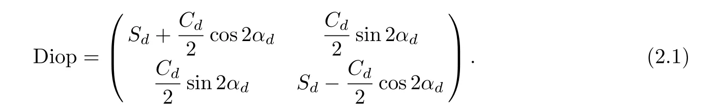
To understand the meaning of this matrix,consider a far point source at the horizontal forward gaze direction.The point emits a spherical wavefront that propagates towards the eye,and then is distorted by the lens two surfaces.Later,this wavefront propagates into the eye,where it is again refracted,this time by the eye’s optical surfaces(cornea,crystalline lens).Since the pupil is relatively small,optometrists consider only the quadratic terms in the Taylor expansion of the wavefront.Indeed Diop is the quadratic form of the second order terms in the wavefront Taylor expansion.The dioptric matrix is,roughly speaking,the shape of the wavefront(after refraction by the spectacles)that would be focused by the person’s eye to a focal point at the retina.Geometrically,Sdis the mean curvature of the wavefront,Cdis the difference between its principal curvatures,andαdis the angle between the principal direction associated with the larger principal curvature and the x axis.In optometry,curvatures are measured in units called diopter,where 1 diopter=1/meter.Therefore,a basic goal is to shape the lens to achieve this prescription dioptric matrix.The problem is that the eye is not looking only at the forward direction;rather,it scans the visual field in many angles.Therefore,it is required to design a lens that would provide dioptric matrices that are as close as possible to the prescription matrix for all gaze directions.

The design paradigm is to consider the“world”as a set of points in space,some far and some near,then,each point emits a spherical wavefront that propagates towards the eye.Computing the wavefront after refraction by the two lens surfaces,we can estimate how close it is to the desired wavefront given by the patient’s prescription.Therefore,there are a few questions we need to answer:

(1)How to compute the refracted wavefront after refraction by the lens?

(2)How to represent the lens surfaces?

(3)Since we need to compromise vision in many gaze directions,what is a good merit function for“good”vision?

(4)What optimization approach to use?This involves convergence,efficiency,accuracy,etc.

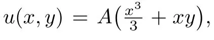
To simplify the analysis,we assume at this point that the lens consists of a single refractive surface,and neglect the refraction by the second surface.We shall remove this assumption in the next section.We further assume that the prescription has no astigmatism,i.e.,Cd=0.In Section 4,we shall explain how to deal with non-zero cylinder.Deviations of the actual power S from the desired power Sd,and nonzero actual cylinder C imply a blurred image on the retina.To minimize that blur,we want to make the expression e=(S−Sd)2+C2small for each gaze direction.However,some directions are more important for normal visual tasks.Therefore,we define the following merit function consisting of a weighted sum of the error e:

where u(x,y)is the refractive surface,S(x,y)and C(x,y)are the actual power and cylinder at a point(x,y),Ωis the projection of the lens surface on the(x,y)plane(the forward direction is denoted z),and wpand wcare given weight functions chosen by designer.Notice that S and C are functions of the surface u.The choice of L2norms for the error is somewhat arbitrary,and other norms are proposed as well.However,it turns out that this norm contributes to the stability of the optimization algorithms;furthermore,designs based on(2.2)and its upgrades described in the next section give rise to excellent lenses.

When the prescription is cylinder-free,it represents locally a spherical wavefront with radius of curvature.The refracted wavefront,needed in the computation of the functional e,is more complicated to compute even if we only consider its local quadratic approximation.Consider first the propagation of the wavefront from its point source Xo=(xo,yo,zo)to the lens surface,along the ray connecting Xowith Xs=(xs,ys,u(xs,ys)).Since we start at a point source,the wavefront is a spherical surface,with curvature,where r=|Xs−Xo|.As a further simplification,we assume in this section that the wavefront hits the surface normally,that is,the baseray(which is normal to the wavefront at its base)is parallel to the normal to the surface u at the point of intersection Xs.If we denote bythe two principal curvatures of the incident wavefront,and bythe two principal curvatures of the surface at Xs,then the principal curvaturesof the refracted wavefront are given by the equation

Here n and n′are the refraction in dices in the media before and after refraction.We shall derive formula(2.3)from a more general result in the next section.

(2.3)implies that up to a suitable constant,the functional e can be written in terms of the surface’s principal curvatures as

where Hsdenotes the mean curvature of the lens surface.

To obtain intuition into the nature of the variational problem of minimizing e(u),consider the canonical homogeneous model wp=wc=1.Upon linearization about a flat surface,u satisfies a bi-harmonic equation:

Based on this observation,Wang et al.proved several regularity results about the minimizers of e.For instance,for clamped boundary conditions they proved the following result.

Theorem 2.1(see[23])Assume u= ∂νu=0 on the boundary ∂Ω,where ∂νdenotes normal derivative.Ifand furthermore wpand wcare bounded from below by a positive constant,then e has a unique minimizer in the Sobolev space H2+k(Ω).

Remark 2.1It is interesting to note that in the special case wp=0,wc=1,the functional e(u)becomes,up to a constant,

where KGis the Gaussian curvature of the surface.Thus e1is essentially the Will more energy of the surface.Moreover,upon linearization about a flat surface,e1becomes

which is the energy of a plate with Poisson ratioσ=−1.While Landau and Lifshitz[13]stated that there are no known substances for whichσis negative,some exotic materials with negative σwere constructed in recent years,and in any case,mathematically the problem is well-defined all the way down toσ=−1.

3 Design Based on Eikonal Functions

The design method presented in the previous section was successfully implemented(see[10])to become one of the leading PALs in the market at the time1Although the patent was issued in 2001,the method was commercially used since the early 90s..However,is it accurate enough?Can it be improved?Two immediate questions come up in this context.Is the approximation of the optical power by surface curvatures good enough?Are we using the correct merit function?

A partial negative answer to the first question was given in[6].The authors computed the optical distance of a set of rays emanating from a point source after refraction by the lens surfaces,and used these distances to construct the refracted wavefront.Their calculation indicated that in some cases the difference between the precise wavefront and its geometric approximation given in equation(2.3)is quite large.We shall therefore upgrade the design method so that the optics of the lens is computed accurately.However,we shall do so by a different method than in[6].One reason for this is that the optimization process requires many iterations,and the use of many free parameters to represent the free form surface.Therefore,the wavefront computation must be very efficient.Another reason is that with the method described below we can capture additional optical features of the lens that are needed for a more general merit function.

The last point is related to the second question we asked.The merit function e in equation(2.2)is based on the minimization of the spread of the image of a point source,namely what is minimized is the image blur at the retina.While this is a very important requirement,one may want to control not only the blur but also the shape of an extended image.For example,quantities such as the local magnification of a small square image,and its distortion also contribute to good vision.

Our method is based on Hamilton’s eikonal function E.This function,and some canonical transforms of it were introduced by Hamilton[8]as the foundation of his geometrical optics theory.

3.1 Eikonal functions

Consider 2 points P=(x,y,z)andin an optical medium characterized by a(possibly varying)refraction index n.The optical distance between the points is the minimal value of the Fermat integralalong all possible paths connecting the two points.We denote it by do(P,P′).The eikonal equation|∇do|=n imposes a constraint on the derivatives of do.It is therefore convenient to restrict the points P and P′to lie on two predetermined surfaces Σ and Σ′,respectively.For example,we select the reference planes(Σ :z=0 and Σ′:z′=0).The choice of the coordinate frames is a bit arbitrary,and might depend on the problem at hand.For instance,if the system has a common optical axis,we may use it as the z and z′axes.The refraction index is n near P and n′near P′.The point eikonal E(x,y,x′,y′)is defined to be the optical distance between P ∈ Σ and P′∈ Σ′.The ray directions are denoted by r=(ξ,η,ζ)and r′=(ξ′,η′,ζ′).It follows from the eikonal equation that the ray directions can be determined from E.For example,

Indeed a main application of E is to determine the associated rays connecting two points in the medium.In the important case where the points are separated by a lens,the point eikonal serves to determine the rays connecting points in the object space(the space near(x,y,z))with points in the image space(the space near(x′,y′,z′)).

It is sometimes preferred to work with a different,more direct characterization of the optical system,provided by a set of equations that determine for each ray in the object space its associated ray in the image space.Using the same notation,we applied for the point eikonal,we look for equations of the form

We term these equations collectively as the lens transformation,or the lens mapping.

There are several reasons for the introduction of objects such as the point eikonal,although the lens transformation seems a more direct way to characterize an optical system.One reason is that eikonals have a transparent geometrical meaning.They are also closely related to the imaging properties of wavefronts as we shall show.Furthermore,certain eikonals are often easier to compute than the lens transformation.Unfortunately,the point eikonal is obviously degenerate for a point object that is focused at an image point.For this reason,Hamilton introduced two more useful eikonal functions.

The point angle eikonal is defined to be the Legendretrans form of E with respect to(x′,y′).We therefore write

Similarly,we define the angle eikonal EA(ξ,η,ξ′,η′)as the Legendre transform of EMwith respect to the variables(x,y):

A great advantage of the angle eikonal is that it changes in a very simple way when we shift either reference plane in the orthogonal direction.Such shifts are important,for example,since we might want to shift a given plane to a new plane where a certain object is imaged.Another instance where shifts are useful is when one wants to study the propagation of wavefronts.Using the analytic definition or the geometric interpretation of the point angle eikonal,it can be shown(see[14])that under an orthogonal shift of the Σ′reference plane by an amount δ′,the point angle eikonal EMis transformed according to

3.2 Local eikonals:Definition and imaging properties

Hamilton’s eikonal functions were rarely used in optical design since their computation is a formidable task,and since in general only part of the information embodied in them is needed.For our purposes,and since as mentioned in the previous section only the local form of the wave should be considered in light of the small pupil,we proceed by defining local eikonals.These functions are far easier to compute,and they contain all the information for the imaging properties of spectacles lenses.

To construct the local eikonals,we consider rays in the vicinity of a base ray that leaves the point P in the direction of the z axis,and arrives at P′along the direction of the normal there z′.In this case,the direction parameters ξ,η,ξ′,η′are zero to first order,and to leading order the point eikonal can be approximated by its quadratic form that is characterized by its Hessian matrix

where P,Q,R are 2×2 matrices.The matrices R and P are symmetric,while Q is not necessarily symmetric.The symmetries of P and R follow from the eikonal equation.

Figure 1 The base ray in the eikonal construction for narrow beams.

We analyze now the optical information encoded in the10 independent parameters that constitute the matrix E.It is convenient to do so by considering separately the matrices P,Q,R.The matrix R determines the classical properties such as power and oblique astigmatism(cylinder).Consider the case where(x,y)=(0,0).Then to leading order,

Figure 2 Top sketch:A line element in the object space,viewed from a point in the image space with no lens in between.Bottom sketch:Same line viewed through an optical element.The information on the change in the viewing directions is stored in the matrix Q.

Multiplying and dividing the last equation by r,we obtain

It follows that the matrixprovides(up to a rigid rotation)the information on the angular magnification of the optical element.We can now define the following geometrical optical parameters:

(1)Angular magnification:

(2)Angular distortion:

(3)Angular magnification angle:ϕ1is the angle of the largest magnification axis.

(4)Torsion:ϕ2is the rotation angle defining the rotation matrix U.

The importance of these quantities to vision was only recently understood(see[2,20]).

3.3 Local eikonals:Computations

We showed in the previous subsection that the local point eikonal E contains not only the blur information of the lens,but also shape information,such as the local magnification and distortion parameters.It remains to develop an efficient method to compute E.We now show how to do so with the help of the angle eikonal EAand the lens transformation introduced in equation(3.1).

For this purpose,we write the Hessians of the local angle eikonal EAand local lens transformation J as

where A,B,···,H are all 2 × 2 matrices.Then the equations for the angle eikonal and lens transformation are

Since the point eikonal E has a similar set of equations,one can easily convert one local eikonal to another.

Since the lens transformation forms a group whose structure is particularly simple in the local approximation we use in this section,we can construct the transformation from a point object into the image space beyond the two lens surfaces as a product:

where I is the 4×4 identity map,J1is the shift transformation from the point source to the anterior lens surface,J2is the refraction transformation through the anterior surface,J3is the shift from the anterior surface to the posterior lens surface,and J4is the refraction transformation through the posterior surface.

The effect of shifting the reference plane on the eikonals can be most conveniently found through the angle eikonal.Expanding equation(3.4)for small angles,we obtain

In terms of the matrix EA,the shift implies

where δ′is the shift,and the matrices A and B remain unchanged under the shift.

The refraction transformation is much harder to compute.In[21],we applied a geometric approach to solve the eikonal equation to obtain a closed expression for J2and J4(see also[22]).Let w be a refractive surface separating a medium with refraction index n and a medium with refraction index n′.Let the incident base ray be r,and the refracted baseray be r′,and let the normal toΣat the hit point of the rays beν.We construct three local coordinate systems(x,y,z),(x′,y′,z′)and(X,Y,Z)for the incident rays,the refracted rays,and the surface Σ,such that the z,z′,Z axes are along r,r′, ν,respectively.Next,we recall from Snell’s law(see[12])that the incident ray,the refracted ray and the surface normal are coplanar.Of course,we also have the Snell relation n sin i=n′sin i′,where i,i′are the angles made by ν and the incident and refracted base rays,respectively.We thus select the x axis to be orthogonal to r in this common plane,with similar choice for x′and X.The third coordinate in each frame is chosen so as to complete the first two coordinates into a regular orthogonal frame.In this coordinate frames,an incident wavefront v about the base ray,the refracted wavefront v′and the refractive surface w are all quadratic functions to leading order.It is convenient to write them down explicitly as

where V,V′,W are 2×2 matrices.

Our goal now is to find the matrices(T,F,G,H)as in equation(3.10)that relate points and directions(x,y,ξ,η)of incident rays on the plane orthogonal to r to points and directions(x′,y′,ξ′,η′)of refracted rays on the plane orthogonal to r′.Without spelling our the details(see[21–22]),we obtain that T,F,H do not depend upon the surface w:

The key information on the refractive surface is found to be encoded in G:

Equations(3.15)–(3.16)are all we need to compute the local lens transformations J2and J4.In addition,equation(3.13)enables the computation on J1and J3.Therefore,we are now able to compute the entire local lens mapping J.As explained above,once J is known,we can invert the eikonal equations to find the imaging matrices R and Q,that contain all the focusing,magnification and distortion parameters of the lens at any point on it.

As a by-product of the formula,we derived for the refraction mapping,we show how to apply it to upgrade Snell’s law.This law relates an incident ray,the refracted ray and the refracting surface normal.Alternatively,Snell’s law relates the tangent planes of the incident wavefront,the refracted wavefront and the refracting surface.We now derive a second order extension of Snell law,by relating the quadratic shapes(V,V′,W)of these surfaces.For this purpose,we observe that for a given incident and refracted wavefronts the ray directions are determined by the ray location on a given plane and the wavefront shape.Using the same notation as above in this subsection,we have the following relations:

Therefore,using the fact that F=0,we obtain

Substituting the expression we obtained for T,G,H in(3.15)–(3.16)into(3.18),we obtain the quadratic refraction formula

In the special case where the incident and refracted wavefronts are both tangent to the refractive surface i=i′=0,equation(3.19)reduces to

which proves the relation(2.3).

3.4 Extended merit function

Now,since we are able to compute the entire matrix E which contains all the imaging properties of a lens at each point,we can upgrade the merit function e of Section 2.

As a first application,consider a design for a person with nonzero cylinder C.It is more convenient in this case to rewrite the dioptric matrix in the form(see[7])

where we introduced the cross cylinders

The notion of cross cylinders is of practical and theoretical importance.Practically,some optometric instruments measure them directly.Theoretically,cross cylinders are natural quantities for expressing both the magnitude and angle of the cylinder.

In analogy with the merit function e defined in Section 2,consider a person with a prescription given by equation(3.21).Assume that one of the lens surfaces is fixed,and the other one u(x,y)is to be optimized.Let Sd(x,y),C+.d(x,y),CX,d(x,y)be a distribution of desired optical power and cross cylinders for the design at a point(x,y).The actual wavefront,or equivalently,actual dioptric component S(x,y),C+(x,y)and CX(x,y)at a point(x,y)can be computed by the method of Subsection 3.3.Then,we define a merit function to be minimized of the form

where

Remark 3.1One may wonder why the desired cross cylinders Cd,+,Cd,Xmay depend upon the position(x,y),while the prescription is a fixed quantity.There are two reasons for that.One reason is that in practice a person does not notice small deviations in cylinder(or power)from his optimal prescription.The designer can exploit this fact to deviate locally in purpose from the prescription in order to achieve an overall good actual optical performance.Another reason is that as the eye rotates it scans the visual field in different directions.This raises an inherent difficulty:The rotation group SO(3)is not commutative,and therefore the cylinder axis seems to depend on the orbit the eye takes from its forward gaze to any given gaze direction!This paradox was resolved in 1845 by the topologist J.B.Listing who postulated the following principle.

Listing’s LawFor each eye there exists a primary visual axis,essentially near the forward looking direction,and an associated primary plane,orthogonal to this axis.All eye rotations from the primary axis to other gaze directions are done by rotating the eye about an axis in the primary plane.

While there is not yet a mechanical foundation to this postulate(in terms of eye muscle geometry),this law was validated,at least approximately,in many tests.

The merit function e(u)can be further extended by including in it terms,such as

where M(x,y)and D(x,y)are the actual magnification and distortion parameters introduced in Subsection 3.2,while Mdand Ddare desired magnification and distortion,e.g.,Md=1,Dd=0.

Op en ProblemWe showed in Section 2 that the functional e(u)defined in equation(2.2)is related to the Will more functional,and its linearization is related to the energy of a plate.In particular,the main operator in the associated Euler-Lagrange equation is biharmonic.There is still no theory,similar to the one presented in[23],for the extended functional e of equation(3.22).An even more challenging problem is to study the functional e of equation(3.22)with the addition of the magnification and distortion terms of equation(3.24).

4 Additional Topics and Op en Problems

4.1 Estimating the cylinder

In the geometric model presented in Section 2 a perfect lens surface would be umbilic with prescribed mean curvature.However,a basic theorem in differential geometry states that the only umbilic surface is a sphere.Thus,if the mean curvature is not constant(and a varying mean curvature is the essence of multifocal lenses),the lens surface cannot be spherical,and therefore it cannot be umbilic.Indeed,while a “perfect” lens is not attainable,we searched for an optimal lens in the sense of the functional e(u),namely,we sought a surface whose mean curvature is close to a given function,while minimizing the surface astigmatism,i.e.,the difference between its principal curvatures.

A very interesting question is what are the inherent limitations of the design.Specifically,we ask the problem as follows.

Op en ProblemFind a lower bound on the astigmatism for a given mean curvature distribution.

While this problem is in general open,a partial result was obtained in this direction by Minkwitz.He proved the result below.

However,since we showed that the geometric properties of the surface only approximate its actual optics,the question is whether a similar estimate on the astigmatism growth can be obtained from information on the power of the lens.Indeed the following result,based on formula derived in[18],holds:

Theorem 4.2(see[17])Consider an incident parallel wavefront that is refracted by a lens surface u(x,y).Let the surface separate media with refraction indices n and n′.Assume without loss of generality that n

where we denote the refracted wavefront astigmatism by Cr(0,y),and Hr(0,y)denotes the wavefront’s mean curvature.

These theorems imply that the lateral growth of the astigmatism away from the center line is twice as fast as the change in the optical power of the lens in the vertical direction.Indeed,essentially all designs of PALs show two regions of relatively high astigmatism just outside a narrow corridor of low astigmatism about the center line.

4.2 Power-adjustable lenses

Recalling that to a first approximation the power of the lens is proportional to its mean curvature,we observe that

Therefore,the shift generated a power change proportional to Aδ.The idea,thus,is to select a cubic surface and parameters,such as A andδ,so that one obtains a desired far vision power in one relative position,and another,near vision power,in the second relative position.

Alvarez’s concept did not meet with commercial success due to poor optical performance.However,this concept was revived recently by Barbero and Rubinstein[3],who used a design methodology as explained in Section 3 above.In the present design,one needs to optimize not only over many gaze directions,but also over two(or more)relative lens shifts,to obtain good optical behavior for all powers.The original goal of[3]was to provide adjustable-power lenses to solve the problem of lack of visual correction that affects over 150 million people in developing countries(see[11]).More recently,the authors showed that the Alvarez-Barbero-Rubinstein(ABR for short)design can be used to provide spectacles for presbyopia that offer for the first time wide field of view at all distances(see[5]).

5 Discussion

We presented the main optical concepts and the associated mathematical methods needed to design high-quality multifocal lenses.Even earlier designs from the 90’s raised fundamental questions in differential geometry;for instance,the open problem put forward in Section 4.The present design paradigm is based on the Hamilton’s eikonal functions.While these functions are the cornerstone of geometrical optics,they were not used before for actual lens design because of their enormous complexity.Spectacles design has become an exception.On the one hand,the eye’s pupil is small relative to the visual field;however,for this reason the eye scans the visual field in a saccadic movement or voluntarily.These facts can be exploited by expressing the effective optical characteristics of the lens via local eikonal functions.

The variational problem of minimizing the functional e defined in equation(3.22)is far harder than the geometrical functional define in equation(2.4).The added functional emdefined in equation(3.24)makes it even harder.Almost nothing is known on these variational problems.

There are many additional aspects of multifocal lens design we did not touch here.One key numerical question is the surface representation.PALs are free form surfaces;namely,they have no symmetry.A number of CAD techniques have been used to represent them,ranging from splines to finite elements.One specific method that was found to be very efficient(among other reasons because of the small pupil)is the method of germs.The surface is defined by the values u(xi,yj)of many anchor points(xi,yj)on it.Then,to approximate u and its first and second derivatives at an arbitrary point,a patch is constructed around this point that includes some of the anchor points to define an approximating local polynomial(germ)of u near the pointThe germ method turns out to be very efficient.Its main drawback is that the patches are not even continuously connected;however,this is not an obstacle,since for manufacturing purposes all,we need to supply the manufacturer is a set of discrete points on the surface u.

While the functionals in(3.22)and(3.24)contain all the local information on the imageblur and image distortion,the actual visual acuity of a person is determined by the eye’s contrast sensitivity.This feature can be greatly affected by scatter in the eye.This problem affects mainly the elderly,but they are natural customers of PALs.A design paradigm that includes a model for contrast sensitivity is still an open problem.

AcknowledgementsThis paper is dedicated to Professor Haim Brezis for his 70th birthday.The author thanks his collaborators Gershon Wolansky,Dan Katzman and Sergio Barbero.He is pleased that Haim himself is using multifocal lensesthat were designed using the principles explained above.

[1]Alvarez,L.,Two-element variable power spherical lens,US Patent,3305294,1967.

[2]Barbero,S.and Portilla,L.,Geometrical interpretation of dioptric blurring and magnification in ophthalmic lenses,Optic Express,23,2015,13185–13199.

[3]Barbero,S.and Rubinstein,J.,Adjustable-focus lenses based on the Alvarez principle,J.Optics,13,2011,125705.

[4]Barbero,S.and Rubinstein,J.,Power-adjustable sphero-cylindrical refractor comprising two lenses,Optical Eng.,52,2013,063002.

[5]Barbero,S.and Rubinstein,J.,Wide field-of-view lenses based on the Alvarez principle,Proc.SPIE 9626,Optical Systems Design;Optics and Engineering VI,2015,962614.

[6]Bourdoncle,B.,Chauveau,J.P.and Mercier,J.L.,Traps in displaying optical performance of a progressive addition lens,Applied Optics,31,1992,3586–3593.

[7]Campbell,C.,The refractive group,Optometry and Vision Science,74,1997,381–387.

[8]Hamilton,W.R.,Systems of rays,Trans.Roy.Irish Acad.15,1828,69–178.

[9]Kanolt,C.K.,Multifocal ophthalmic lenses,US Patent,2878721,1959.

[10]Katzman,D.and Rubinstein,J.,Method for the design of multifocal optical elements,US Patent,6302540,2001.

[11]Kealy,L.and Friedman,D.S.,Correcting refractive error in low income countries,British Medical J.,343,2011,1–2.

[12]Keller,J.B.and Lewis,R.M.,Asymptotic methods for partial differential equations:The reduced wave equation and Maxwell’s equations,Surveys in Applied Mathematics,1,1993,1–82.

[13]Landau,L.D.and Lifshitz,E.M.,Theory of Elasticity,Pergamon Press,New York,1986.

[14]Luneburg,R.K.,The Mathematical Theory of Optics,UCLA Press,California,1964.

[15]Maitenaz,B.F.,Ophthalmic lenses with a progressively varying focal power,US Patent,3687528,1972.

[16]Minkwitz,G.,Uber den Flachenastigmatismus Bei Gewissen Symmetruschen Aspharen,Opt.Acta,10,1963,223–227.

[17]Rubinstein,J.,On the relation between power and astigmatism of a spectacle lens,J.Opt.Soc.Amer.,28,2011,734–737.

[18]Rubinstein,J.and Wolansky,G.,A class of elliptic equations related to optical design,Math.Research Letters,9,2002,537–548.

[19]Rubinstein,J.and Wolansky,G.,Wavefront method for designing optical elements,US Patent,6655803,2003.

[20]Rubinstein,J.and Wolansky,G.,Method for designing optical elements,US Patent,6824268,2004.

[21]Rubinstein,J.and Wolansky,G.,A mathematical theory of classical optics,in preparation.

[22]Walther,A.,The Ray and Wave Theory of Lenses,Cambridge University Press,Cambridge,1995.

[23]Wang,J.,Gulliver,R.and Santosa,F.,Analysis of a variational approach to progressive lens design,SIAM J.Appl.Math.,64,2003,277–296.