Gang TIAN

(Dedicated to Haim Brezis on the occasion of his 70th birthday)

1 Introduction

In this note,we extend a third derivative estimate in[4]to Monge-Ampere equations in the conic case.For the purpose of our application,we will consider the complex Monge-Ampere equations in this note.The same result holds for real Monge-Ampere equations.

Let U be a neighborhood of(0,···,0),and u satisfy

and

whereβ∈(0,1)andωβis the standard conic flat metric on Cn:

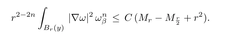
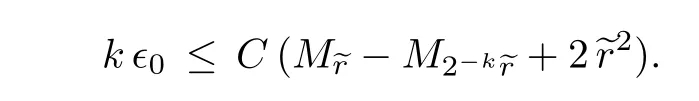
Theorem 1.1Let V be an open neighborhood of(0,···,0),whose closure is contained in U.Then for any α 0 and Cα,which may depend on α,c0,V,inf∆F and∥F∥C1,such that for any x∈ V and 0

where Br(x)denotes the ball with center x and radius r,∇ is the covariant derivative,∆ denotes the Laplacian and the norm is taken with respect to ωβ.

It follows from Theorem 1.1 and the standard arguments,e.g.,by using the Green function.

Corollary 1.1Let u and F be as in Theorem 1.1.Then for any α ∈ (0,β−1− 1)and α<1,is Cα-bounded with respect to ωβ.

This corollary was used by Jeffres-Mazzeo-Rubinstein in their proving the existence of Kähler-Einstein metrics with conic singularities.We refer the readers to Appendix B of[3]for details.

Theorem 1.1 has been known to me for some time.The proof is identical to that in[4].Its arguments were inspired by Giaquinta-Giusti’s work(see[2])on harmonic maps.For years,I had talked about this approach to the C2,α-estimate for complex Monge-Ampere equations in my courses on Kähler-Einstein metrics.

2 The Proof of Theorem 1.1

In this section,we prove Theorem 1.1 by following the arguments in Section 2 of[4].I will present the proof for complex Monge-Ampere equations in details.In[4],the proof was written for real Monge-Ampere equations,though it also applies to complex Monge-Ampere equations.

Without loss of generality,we may assume x∈V∩{z1=0}.In fact,one can apply known estimates(see,e.g.,[4])to u outside the singular set{z1=0}ofωβ.If F is smooth on U,we can also apply Calabi’s third derivative estimate to u outside{z1=0}(see[5]).

Define Bβ(r)to be the domain in C × Cn−1consisting of all(w1,w′),where w′=(w2,···,wn),satisfying

There is an r>0 such thatand w′=(z2,···,zn)defines a natural map frominto U.This map is isometric from the interior ofonto its image.For convenience,we will use w1,···,wnas coordinates.By scaling,we may assume thatr=1.

In terms of coordinates w1,···,wn,we have

and covariant derivatives of u become ordinary derivatives,e.g.,

We will denote det(ukl)uijby Uij,where(uij)denotes the inverse of

First we recall two elementary facts.

Lemma 2.1(see[4,Lemma 2.1])For each j,where all derivatives are covariant with respect to ωβ.

ProofRecall the identities

Differentiating them in wk-direction and summing over k,we get

Then the lemma follows.

Lemma 2.2(see[4,Lemma 2.2])For any positive λ1,···,λn,we have

where λ = λ1···λn,and C is a constant depending only on λiand

ProofIn[4],(2.2)is proved by the properties of determinants.Here we outline a simpler proof.First by using the homogeneity and positivity of,we only need to prove the case whenNext,if we denote the left-hand side of(2.2)by f(Λ),then by a direct computation,for i=1,···,n.Then(2.2)follows from the Taylor expansion of f at I.

In terms of w1,···,wn,(1.1)becomes

By a direct computation,we deduce from this

This system resembles the one for harmonic maps whose regularity theory were studied extensively in 70s and 80s.The idea of[4]is to apply the arguments,particularly in[2],from the regularity theory for harmonic maps.

The following lemma follows easily from the Sobolev embedding theorem.

Lemma 2.3There is a constant Cβ,which depends on β,such that for any smooth function h on Bβ=Bβ(1)with boundary condition

we have

Note that Cβblows up whenβtends to 1.

Lemma 2.4(see[4,Lemma 2.3])There is some q>2,which may depend on β,and,such that for any,we have

whereand C denotes a uniform constant.1Note that C,c always denote uniform constant though their actual values may vary in different places.

ProofFirst we assume y=x.Defineλijby

By using unitary transformations if necessary,wemay assumefor anyand i,j ≥ 2.It follows from(1.2)that

where I denotes the identity matrix.

Choose a cut-off function η:Br(x)7→ R satisfying

Using Lemma 2.1 and(2.4),we can deduce

whereand λ = λ1···λn.

Using Lemma 2.1,we have

Then by Lemma 2.2,we can deduce from the above that

By applying the Sobolev inequality to(i,j ≥ 2)and Lemma 2.3 toin the above,we get

This inequality still holds,if we replace Br(x)by any Br(y)which is disjoint from the singular set{z1=0}.This can be proved by using the same arguments,but Lemma 2.3 is not needed.One can easily deduce from this and a covering argument that for any ball B2r(y)⊂U,

Then(2.7)follows from Gehring’s inverse Hölder inequality(see[1]).

Lemma 2.5(see[4,Lemma 2.4])For any y∈V and B4r(y)⊂U andσ

Multiplying(2.10)bywe get

It follows that

Multiplying(2.4)by b w and integrating by parts,we have

Using the assumption that∇F is bounded,we can easily deduce from this

By Lemma 2.4 and the Poincare inequality,we have

Without loss of generality,we may assume that q≥2(q−2).Sincevanishes on∂Br(y),its L2-norm is controlled by the L2-norm ofand consequently,of|∇ω|.Then we have

Next,we recall a simple lemma which can be proved by standard methods.

Lemma 2.6Let h be any harmonic function on Bβ=Bβ(1),such that

Then for any r<1,

In fact,we only need a weaker version of Lemma 2.6 in the subsequent arguments:In addition to the assumption(2.15),we may further assume

Remark 2.1If we replace(2.15)by

then we have a better estimate

We observe

Hence,by(2.11)and(2.18),we get

Clearly,(2.9)follows from(2.12)–(2.14)and(2.19).

In view of(2.9),we need the following lemma.

Lemma 2.7(see[4,Lemma 2.5])For any ϵ0>0,there is an ℓdepending only on ϵ0,and inf∆F satisfying that for any e r>0 with Ber(y)⊂ U,there issuch that

ProofIt follows from(2.4)that

where∆′denotes the Laplacian ofω.

Letηbe a non-negative function on Br(y)satisfying thatη(z)=1 for anyη(z)=0 for any z near ∂Br(y)andThen

where

SetIt follows from(2.21)that for a suitable constanti.e.,Z is super-harmonic with respect toω.Sinceω is equivalent toωβ,we can apply the standard Moser iteration to∆′to get

It follows that

Hence,if(2.20)does not hold forthen

This is impossible if k is sufficiently large.So the lemma is proved.

Now we complete the proof of Theorem 1.1.Chooseξ=λ2αandλ∈(0,1),such that

Next we chooseϵ0and r0sufficiently small,such that

Then we can deduce from(2.9)that forσ=λr and r≤r0satisfying(2.20),

whereν = β−1−1>α.Then(1.3)follows again from this and a standard iteration.

[1]Gehring,W.,The Lp-integrability of the partial derivatives of a quasiconformal mapping,Acta Math.,130,1973,265–277.

[2]Giaquinta,M.and Giusti,E.,Nonlinear elliptic systems with quadratic growth,Manuscripta Math.,24(3),1978,323–349.

[3]Jeff res,T.,Mazzeo,R.and Rubinstein,Y.,Kähler-Einstein metrics with edge singularities(with an appendix by C.Li and Y.Rubinstein),Annals of Math.,183,2016,95–176.

[4]Tian,G.,On the existence of solutions of a class of Monge-Ampere equations,Acta Mathematica Sinica,4(3),1988,250–265.

[5]Yau,S.T.,On the Ricci curvature of a compact Kähler manifold and the complex Monge-Ampere equation,I,Comm.Pure Appl.Math.,31,1978,339–411.