A fast real non-local means methodfor image denoising

2016-12-22WUShiqianYANGChaoJIANGJunZENGLiangcai

西安邮电大学学报 2016年6期

WU Shiqian, YANG Chao, JIANG Jun, ZENG Liangcai

(1.School of Machinery and Automation, Wuhan University of Science and Technology, Wuhan 430081, China;2.Hubei Collaborative Innovation Center for Advanced Steels, Wuhan University of Science and Technology, Wuhan 430081, China)

WU Shiqian1,2, YANG Chao1, JIANG Jun1, ZENG Liangcai1

Large computation is an issue for Non-Local Means (NLM) method. A fast method is proposed to implement the NLM method by representing patches in terms of features so that each patch is computed only one time. Unlike the previous methods, the metric for patch similarity is the same measure as used in NLM instead of heuristic thresholds. 2D histogram and summed-area table are employed to speed up searching similar patches. Moreover, a patches-based method is developed to blindly estimate noise level for filtering parameter. The proposed method achieves NLM solution in entire image. Experiments carried on Tampere Image Database (TID) demonstrate that the proposed method outperforms the semi-local implementation, which restricts patch search in a local neighborhood.

image denoising, non-local means, patch features, 2D histogram, summed-area table

CLC Nubmer: TN911.73 Document Code: A Article ID: 2095-6533(2016)06-0007-07

Denoising has been one of the fundamental problems in image processing. Buades et al provided a review on denoising algorithms[1], in which one emerging denoising technique is the non-local means (NLM) method[1-2]. The NLM idea is to use redundant information of images to reduce additive noise. It has been shown that the NLM algorithm provides state-of-the-art results in both PSNR and visual quality. However, the superior performance of the NLM algorithm is achieved at cost of huge computation. For an image with size M×M, selecting the patch size as B×B, the computational complexity of the NLM method is O(B2M4), which is too expensive to be used in practical applications.

To reduce computation, Buades et al[2]proposed to search similar patches in a relatively large “search window” of size S×S instead of the whole image, which modifies the initially NLM method into a semi-local means (SLM) solution. The computational complexity is then reduced to O(S2B2M2). Recently, various NLM speed-up approaches have been introduced, which can be classified into three categories: 1) fast operators, for example, using FFT[3], convolution[4]; 2) data-driven lower dimensional subspace of image neighborhoods, such as using SVD[5]or PCA[6]; 3) pre-selection methods, i.e., eliminating dissimilar pixels in computation. The typical criteria for pre-classification include mean and gradient[7], mean and variance[8-9], moments[10]or cluster tree[11].

The proposed method belongs to the third category mentioned above. Different from previous approaches[7-10], the proposed criteria for patch pre-classification are derived from Euclidean distance of patches. As such, the similarity measurement is based on identical metric in paper [11], but the computation of [11] is still expensive. More importantly, the proposed method has no pre-defined thresholds as previous approaches[7-8,10]did. Another contribution of this paper is to propose a blind method to estimate noise level from a single image.

In the following section, a fast scheme to implement the NLM method is proposed. Section 2 presents a blind method for noise estimation. Section 3 demonstrates experimental results carried on Tampere Image Database (TID)[12], followed by conclusion in Section 4.

1 Efficient scheme for NLM method

1.1 NLM method

Considering a noise image I∈M×M, the output of NLM method is computed as follows[2]:

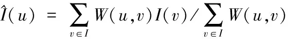
(1)

where W(u, v) is a weight assigned to pixel u with respect to pixel v, according to similarity between two patches P(u),P(v)∈B×Bcentered at u and v respectively:

(2)

where h is the filtering parameter which is proportional to noise variance. Obviously, the NLM algorithm works by averaging pixels while the weights depend on their similarity with the pixel of interest. It is seen from equations (1) and equations (2) that enormous computation comes from calculating weights. For each pixel, M2weights for NLM (or S2for SLM) algorithm are calculated. Accordingly, there are M4weights for entire image. If each patch is represented by features and pre-computed individually, patch computation is M2times, which reduces computational complexity significantly.

1.2 Representing Euclidean distance of patches in terms of statistical features

Given a reference patch P(u), the Euclidean distance between P(u) and arbitrary patch P(x) is

d(P(u),P(x))=‖P(u)-P(x)‖2=

E{[P(u)-P(x)]2}=

E{[P(u)-E(P(u))-

P(x)+E(P(x))+

E(P(u))-E(P(x))]2}=

[E(P(u))-E(P(x))]2+

var(P(u))+var(P(x))-

2cov[P(u),P(x)].

(3)

where E(P(u)), var(P(u)) are mean and variance of P(u) respectively, cov(P(u),P(x)) is the co-variance of P(u) and P(x). Noticing the following statistical relationship:

var(P(u))=[S(P(u))]2,

(4)

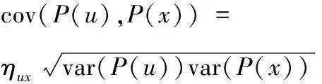
(5)

where ηuxis the correlation coefficient of P(u) and P(x), S(P(u)) is the standard deviation (std) of P(u), and replacing equations (4) and (5) into equation (3), we derive

(6)

The patches which are most similar to reference patch P(u) are those with the following features

E(P(x))=E(P(u)),

(7)

S(P(x))=ηuxS(P(u)).

(8)

Therefore, the similar patches could be completely found by their statistical features, i.e., mean, std and correlation coefficient.

Unlike the correlation coefficient, the E(P(x)), S(P(x)) can independently be computed and stored. However, the parameter ηux⊂[0,1] is also an indicator of patch similarity, in which two patches are similar when ηuxis large. Accordingly, the search of similar patches can be started by setting ηuxas 1. i.e., find the patches which satisfy:

1) E(P(x)) = E(P(u)),

2) S(P(x)) = S(P(u)).

If insufficient patches are found, ηuxis reduced to seek more similar patches. Obviously, the issue of finding similar patches is a search strategy. In the following, 2D histogram and summed-area table are proposed to fast search similar patches.

1.3 2D histogram to represent statistical features

E(i,j)=E1,

S(i,j)=S2.

The 2D histogram directly reveals the distribution of patch features.

Fig.1 2D histogram of mean (E) and std (S)

1.4 Summed-area table for fast searching similar patches

For a specific patch Pi, the number of similar patches can be found from 2D histogram directly. If few similar patches are found, searching sufficient similar patches in whole feature domain iteratively is time-consuming. Thus, the summed-area table[13]is employed to improve search speed.

A summed-area table, denoted SAT(x,y) represents the sum of values located in upper left rectangular region of location H(x, y), which is defined as follows[13]:

(9)

As shown in Fig.2, the sum of a rectangular region can be easily obtained by

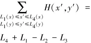
(10)

It is seen from equation (10) that the search of similar patches by summed-area table is only three addition and subtraction operations.

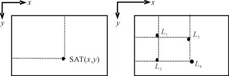
(a) summed-area table (b) sum of a rectangular region

Fig.2 Summed-area table and computation

2 Estimation of noise level

As mentioned in section 1.1, the parameter h in equation (2) acts as filtering parameter which depends of noise level[1-2]. Large h results in blurring, while a small h affects denoising performance. Here, a patch-based method is developed to blindly estimate noise level from a single image.

Suppose the noise is independent and identically-distributed with zero mean Gaussian noise, given by

I(x,y)=I0(x,y)+n(x,y),

(11)

where I(x,y), I0(x,y) and n(x,y) are noisy image, ideal image and noise respectively. The goal of noise estimation is to obtain noise variance (std) from noisy image I(x,y). To this end, filter-based method[14],patch-based (segmentation) method[15], and hybrid-based method[16]have been proposed. A special method based on characteristics of natural images was introduced in [17]. The idea of patch-based method is to divide an image into a set of overlapped or non-overlapped patches. The local variance of homogeneous blocks is then viewed as the noise variance.

Assume overlapped patches P(u) (u=1,2,…,M2) are obtained. It is tough to judge which patch is most homogeneous for noise estimation because image content cannot be separated from noise. We notice that edges are remarkable contents of images. Accordingly, edge detection is employed as homogenous analyzer. In this work, Canny detector is used because it is robust to noise.

Let Q(u) be the set of patches without edges. It is noted that edges are not the only content. To further alleviate the effect of image content, we borrow the idea of noise level function (NLF), i.e., noise variance is defined as function of brightness[15], and a robust method is proposed to extract noise level from homogenous patches in different grayscale levels.

Computing mean E(i) and std S(i) of homogenous patches Q(i) (i=1,2,…,NH), for brightness E=Cj, find

(12)

and obtain the histogram

Gj(k)={gj(1),gj(2),…,gj(nj)}.

(13)

Furthermore, we find

(14)

The noise level in brightness Cjis determined by

(15)

with confidence

(16)

Then, the final noise level is weighted average by the estimated std values with the top 5 confidence as follows:

(17)

3 Experimental result

In this section, experiments have been performed to test the proposed method based on TID databse shown in Fig. 3. The database consist of 25 images, and all images are of size 384×512. The patch size used for noise estimation and denoising is 7×7, as recommended in [1-2]. All experiments are performed on Dell workstation T7400 (Q-Core Xeon, 3.2G) in Matlab environment.

Fig.3 Test images in TID database

3.1 Noise estimation

Gaussian noises with zero mean but in different levels (S = 5, 10, 15, …, 40) are injected into original images. The estimation is directly carried on each noisy image. The average results on 25 images of the proposed method in comparison with methods of [14-17] are shown in Fig.4.

It is observed that methods in [15, 17] are accurate if noise level is low, but their performances are not robust. For method in [14], it is over-estimation and under-estimation with respect to low and high noise levels[14,16]. The proposed method provides better estimation than [16], which provides state-of-the-art results.

Fig.4 Estimated noise levels in different methods

3.2 Image denoising

It is observed from Table 1 that the proposed method achieves better results than the SLM method. Results shown in Fig. 5 demonstrate that our method achieves higher PSNR in 20 of the database, especially for image 25 (2.98 dB increase) and image 13 (1.84 dB increase).

Fig.5 PSNR results by different methods

Fig.6 Operation times by different methods

MethodSLM[8][10]OurmethodAveragePSNR32．6832．2232．7532．95Averagetime419．63298．91241．3281．5

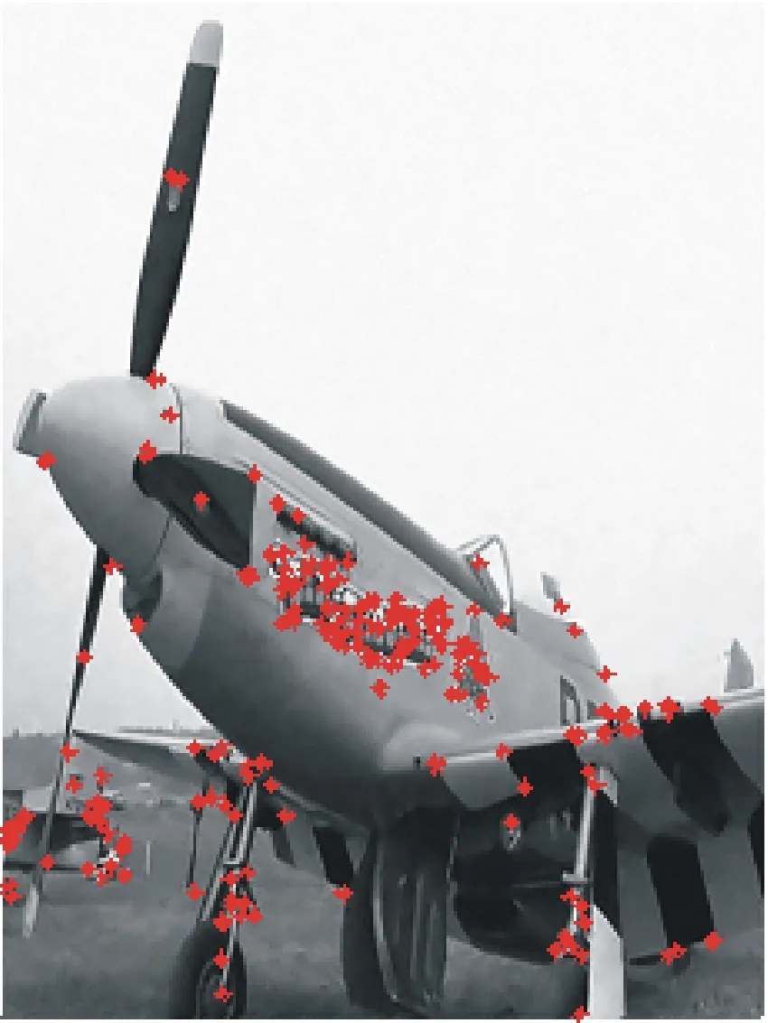
It is also noticeable that there is a decrease in the PSNR values by the proposed method for images 3 (caps), 4 (lady), 7 (window and flower), 15 (girl) and 20 (plane), in which the image 20 has biggest decrease (1.01 dB). Carefully analyzing these images, it is observed that these image contents are generally smooth with low texture, and therefore contain lots of similar features in entire images (for example, the sky in image 20 shown in Fig. 7). Further study reveals that bigger error produced by the proposed method mainly happens on edges marked as “*” shown in Fig. 7(d). By studying the denoised images, it can be observed that the visual quality by the proposed method is more pleasing as highlighted in part of Fig.7.

It is seen from Fig. 6 that the proposed method is generally more efficient than the SLM, while the operation time by the SLM is very stable and consistent because the operation for each pixel is always O(S2B2). It is also observed that the proposed method spends more time on images 2 and 20. The operation for each pixel by the proposed method is O(NB2) where N is number of similar patches. If large similar features are found, for example, N≫S2for sky part in image 20, the speed of the proposed method is slow. The experiments reveal that the proposed method is very suitable for complex images with rich contents.

(a) noisy image

(b) denoising results (SLM)

(d) big error marked

Fig.7 Comparison of Denoising results

The proposed method is closely related to methods in [7-11]. The method in [11] arranges data in tree structure which needs cross comparison. The methods in [7-10] need several thresholds for feature selection, whereas our method has only one threshold Nminwhich offers tradeoff between accuracy and efficiency. The method in [7] employs gradient information, which is sensitive to noise and computationally complex[8]. The PSNR and operation time for methods in [8, 10] are shown in Fig.5, Fig.6 and Table 1. Results indicate that the proposed method outperforms of [8, 10] in PSNR only except images 20 and 25. Especially, the proposed method is much more efficient than the methods in [8, 10]. In contrast to methods in [7-8, 10], our method essentially adopts flexible thresholds which depends of image contents. In [9], the authors try to improve accuracy of [8] by using wider thresholds. Using these thresholds, the operation time tested by an image (cameraman) with size 128 × 128, is 5 370.9 second, so that this method can only work in SLM scheme as shown in [9].

4 Conclusion

A fast NLM method working in entire image is introduced in this paper. The method comprises two parts: noise estimation and noise removal. A patch-based method is developed to estimate noise level from a single image. A theoretical derivation to represent Euclidean distance of patches in terms of patch statistical features is shown. This allows reduction of computation complexity to O(NB2M2). To speed up searching similar patches, 2D histogram and summed-area table are employed. Experiments on TID database show that the proposed method not only reduces computational burden, but also improves denoising performance due to full use of image information. The proposed method significantly outperforms the SLM solution for the images with rich context.

Reference

[1] BUADES A, COLL B, MOREL J M. A review of image denoising algorithms, with a new one[J/OL]. Siam Journal on Multiscale Modeling & Simulation, 2005, 4(2):490-530[2016-05-06].http://dx.doi.org/10.1137/040616024.

[2] BUADES A, COLL B, MOREL J M. Nonlocal image and movie denoising[J/OL]. International Journal of Computer Vision, 2008, 76(2):123-139[2016-05-06].http://dx.doi.org/10.1007/s11263-007-0052-1.

[3] WANG J, GUO Y, YING Y, et al. Fast non-local algorithm for image denoising[C/OL]//2006 IEEE International Conference on Image Processing. [S.l.]:IEEE, 2006:1429-1432[2016-05-06]. http://dx.doi.org/10.1109/ICIP.2006.312698.

[4] CONDAT L. A simple trick to speed up and improve the non-local means[J/OL]. Image (Rochester, N.Y.), 2010,2(7):1-3[2016-05-06].https://www.mendeley.com/catalog/simple-trick-speed-up-improve-nonlocal-means.

[5] ORCHARD J, EBRAHIMI M, WONG A. Efficient nonlocal-means denoising using the SVD[C/OL]//Proceedings of 15th IEEE International Conference on Image Processing. [S.l.]:IEEE,2008:1732-1735[2016-05-06]. http://dx.doi.org/10.1109/ICIP.2008.4712109.

[6] TASDIZEN T. Principal neighborhood dictionaries for nonlocal means image denoising[J/OL]. IEEE Transactions on Image Processing, 2009, 18(12):2649-2660[2016-05-06]. http://dx.doi.org/10.1109/tip.2009.2028259.

[7] MAHMOUDI M, SAPIRO G. Fast image and video denoising via nonlocal means of similar neighborhoods[J/OL]. IEEE Signal Processing Letters, 2010, 12(12):839-842[2016-05-06]. http://dx.doi.org/10.1109/LSP.2005.859509.

[8] COUPE P, YGER P, BARILLOT C. Fast non local means denoising for 3D MR images[C/OL]//Medical Image Computing and Computer-Assisted Intervention - MICCAI 2006:9th International Conference, Copenhagen, Denmark, October 1-6, 2006. Proceedings, Part II. Berlin:Springer-Verlag Berlin Heidelberg,2006:33-40[2016-05-06].http://dx.doi.org/10.1007/11866763_5.

[9] COUPE P, YGER P, PRIMA S, et al. An optimized blockwise nonlocal means denoising filter for 3-D magnetic resonance images[J/OL]. IEEE Transactions on Medical Imaging, 2008, 27(4):425-441[2016-05-06]. http://dx.doi.org/10.1109/TMI.2007.906087.

[10] DAUWE A, GOOSSENS B, LUONG H, et al, A fast non-local image denoising algorithm[C/OL]//Proceedings of SPIE 6812, Image Processing: Algorithms and Systems VI.San Jose: SPIE,2008:1331-1334[2016-05-06]. http://dx.doi.org/10.1117/12.765505.

[11] BROX T, KLEINSCHMIDT O, CREMERS D. Efficient nonlocal means for denoising of textural patterns[J/OL]. IEEE Transactions on Image Processing, 2008, 17(7):1083-1092[2016-05-06].http://dx.doi.org/10.1109/TIP.2008.924281.

[12] Tampere Image Database 2008 (TID 2008)[DB/OL].[2016-05-06]:http://www.ponomarenko.info/tid2008.htm.

[13] CROW F C. Summed-area tables for texture mapping[J/OL]. ACM Siggraph Computer Graphics, 1984, 18(3):207-212[2016-05-06]. http://dx.doi.org/10.1145/800031.808600.

[14] IMMERKAR J. Fast noise variance estimation[J/OL]. Computer Vision & Image Understanding, 1996, 64(2):300-302[2016-05-06]. http://dx.doi.org/10.1006/cviu.1996.0060.

[15] LIU C, SZELISKI R, KANG S B, et al. Automatic estimation and removal of noise from a single image[J/OL]. IEEE Transactions on Pattern Analysis & Machine Intelligence, 2008, 30(2):299-314[2016-05-06].http://dx.doi.org/10.1109/TPAMI.2007.1176.

[16] YANG S M, TAI S C. A design framework for hybrid approaches of image noise estimation and its application to noise reduction[J/OL]. Journal of Visual Communication & Image Representation, 2012, 23(5):812-826[2016-05-06]. http://dx.doi.org/10.1016/j.jvcir.2012.04.007.

[17] ZORAN D, WEISS Y. Scale invariance and noise in natural images[C/OL]//2009 IEEE 12th International Conference on Computer Vision. [S.l.]:IEEE,2009:2209-2216[2016-05-06].http://dx.doi.org/10.1109/ICCV.2009.5459476.

[Edited by: Chen Wenxue]

一种快速非局部均值图像去噪方法

伍世虔1,2，杨超1，蒋俊1，曾良才1

(1.武汉科技大学机械自动化学院, 湖北武汉 430081; 2. 武汉科技大学湖北省高性能钢铁协同创新中心, 湖北武汉 430081)

针对非局部均值(NLM)去噪算法运算量大的缺点，给出一种快速NLM方法。通过特征来表示块的信息，使每个块只计算一次，从而减少计算时间。与先前的方法相比，所给方法的相似性度量准则与NLM方法一致，且不需要预先设置阈值。为加速相似块的搜索，采用2D直方图和积分图两种方法。另外，给出基于块的方法对图像噪声进行盲估计，以求解滤波参数。针对坦佩雷图像数据库(TID)所进行的实验结果表明，所给方法利用整幅图像信息，故其性能明显优于半局部均值(SLM)算法。

图像去噪；非局部均值；块特征；二位直方图；积分图

10.13682/j.issn.2095-6533.2016.06.002

Received on：2016-07-22

Supported by：The National Natural Science Foundation of China under Grant (61371190)

Contributed by：Wu Shiqian (1964-), male, Ph. D degree, Professor, engaged in computer vision, pattern recognition, fuzzy system and neural networks. E-mail:shiqian.wu@wust.edu.cn Yang Chao (1992-), male, postgraduate, research in mechanical engineering. E-mail:1925993033@qq.com