Liangcai MEI (梅良才)

Zhuhai Campus, Beijing Institute of Technology, Zhuhai 519088, China

E-mail: mathlcmei@163.com

Abstract In this article, a new algorithm is presented to solve the nonlinear impulsive dif-ferential equations. In the first time, this article combines the reproducing kernel method with the least squares method to solve the second-order nonlinear impulsive differential equations.Then, the uniform convergence of the numerical solution is proved, and the time consuming Schmidt orthogonalization process is avoided. The algorithm is employed successfully on some numerical examples.

Key words Nonlinear impulsive differential equations; Broken reproducing kernel space;numerical algorithm

1 Introduction

In recent years, the impulsive differential equation model has been applied to many as-pects of life: population dynamics [1], physics, chemistry [2], irregular geometries and interface problems [3–5], and signal processing [6, 7]. Many scholars studied the existence and numerical solution of the impulsive differential equations [8–13]. Y. Epshteyn [14] solved the high-order linear differential equations with interface conditions based on Difference Potentials approach for the variable coefficient. However, so far, no scholars have discussed the numerical solution of the second-order nonlinear impulsive differential equations. Only a few scholars studied the existence of solutions [15]. A. Sadollaha [16] suggested a least square algorithm to solve a wide variety of linear and nonlinear ordinary differential equations. R. Zhang [17] presented the reproducing kernel method and least square to nonlinear boundary value problems. These research work shows that the least square method plays a very good role in solving nonlinear problems. As known to all, the reproducing kernel method is a powerful tool to solve differential equations [17–21]. Al-Smadi M. [22–27] introduced a iterative reproducing kernel method and other methods for providing numerical approximate solutions of time-fractional boundary value problem.

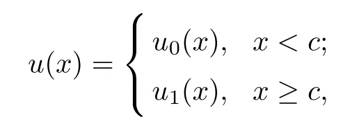
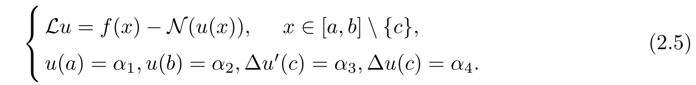
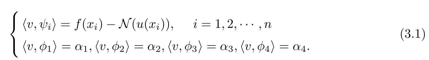
In this article,we consider the following second-order nonlinear impulsive differential equations(NIDEs for short):

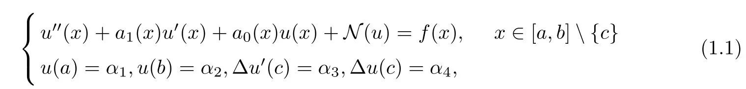
where ∆u′(c) = u′(c+)−u′(c−), α3and α4are not at the same time as 0, ai(x) and f(x) are known function, N : R →R is a continuous function, and αj∈R,j = 1,2,3,4. In this article,only one pulse point is considered, and by that analogy, the algorithm can also be applied to multiple pulse points.

The aim of this article is to derive the numerical solutions of Equation (1.1)in Section 1.In Section 2, we introduce the reproducing kernel space for solving problems. The reproducing kernel method and the least squares method are presented in Section 3. In Section 4, the presented algorithms are applied to some numerical experiments. Then, we end with some conclusions in Section 5.

2 The Broken Reproducing Kernel Space

In this article, the traditional reproducing kernel space is dealt with delicately, and the space has been broken into two spaces that each one is smooth reproducing kernel space,so we can use this space to solve NIDEs. We assume that Equation (1.1) has a unique solution.

2.1 The traditional reproducing kernel space

The reproducing kernel spaces areandwith reproducing kernel(x) and(x),respectively.

In the same way,the reproducing kernel spaces are[c,b](for short)and[c,b](for short) with reproducing kernel(x) and(x), respectively.

2.2 The reproducing kernel space with piecewise smooth

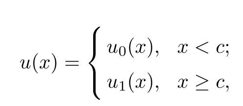
In this article, consider that the exact solution of Equation (1.1) is not a smooth function,so, we connected two reproducing kernel spaces on both sides of the impulsive point, and we call it the broken reproducing kernel space. We have proposed this method for the first time.

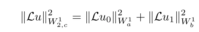
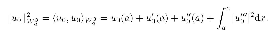
Definition 2.1The linear space W32,cis defined as

Theorem 2.1Assuming that the inner product and norm in[a,b] are given by

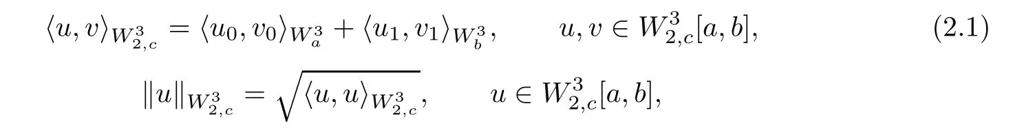
ProofFor any u,v ∈[a,b],

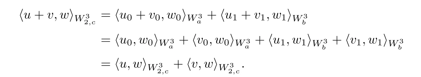
We can prove that the Equation (2.1) satisfies the other requirements of the inner product space.

Theorem 2.2The space[a,b] is a Hilbert space.

ProofSuppose that {un(x)}is a Cauchy sequence in[a,b], however,

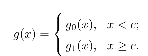
So, there are two functions g0(x)∈, g1(x)∈, such that

Let

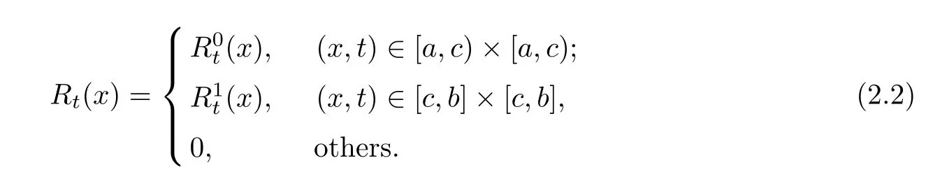
Theorem 2.3The space[a,b] is a reproducing kernel space with the reproducing kernel function

ProofConsider arbitrary u(x)∈[a,b].

In conclusions, for every u(x)∈[a,b], it follows that

Similarly, the reproducing kernel space[a,b] is defined as

and it has the reproducing kernel function

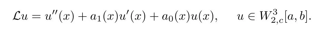
In order to solve Equation (1.1), we introduce a linear operator

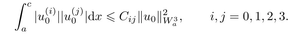
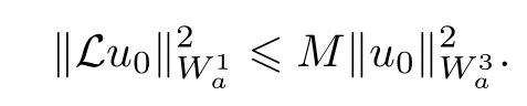
Theorem 2.4L is a bounded operator.

ProofFor each fixed u(x)∈[a,b], by Difinition 2.1, u(x) has the following form

Moreover,

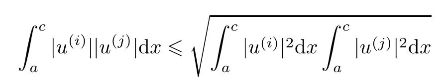
and

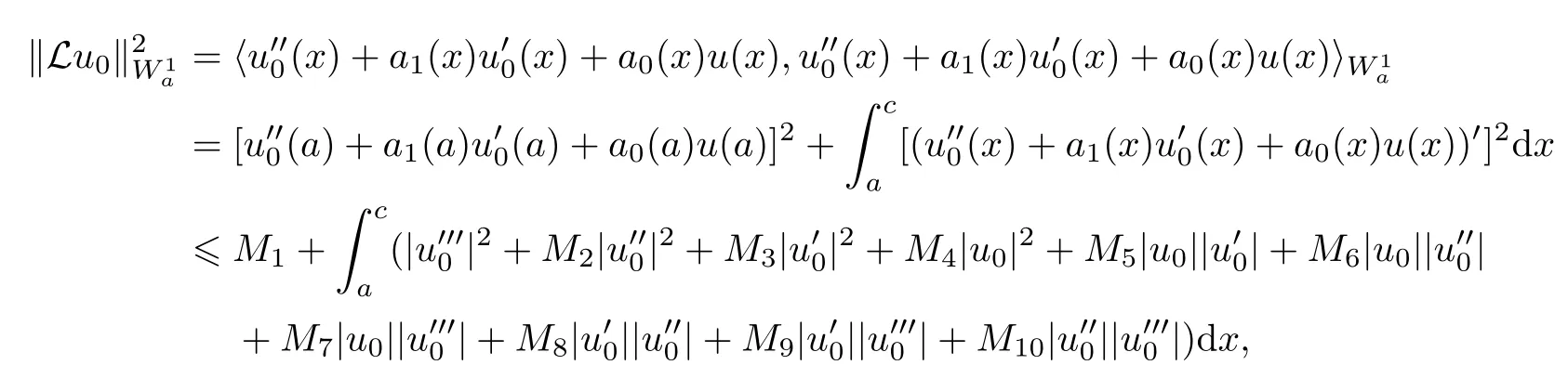
where Mi(1≼i≼10) are constants.

Furthermore,

and

So,

Therefore,

Where M and Cij(i,j =0,1,2,3) are constants.

As a result,

In other words, L is a bounded opertor.

Then, Equation (1.1) can be transformed into the following form:

and

where L∗is the adjoint operator of L.

The orthogonal projection operator is denoted by Pn:[a,b]→Sn, and let

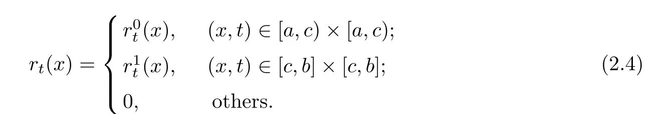
Theorem 2.5ψi(x)=LRx(xi), i=1,2,··· .

Proof

Theorem 2.6For each fixed n,is linearly independent in[a,b].

ProofLet

Similarly, we have k1=0,k2=0, and k4=0.

So, λj=0,j =1,2,··· ,n.

3 Primary Result

In this section, by the least square method, the approximate solution of Equation (2.5)is presented in the broken reproducing kernel space[a,b]. And the convergence of the approximate solution is proved.

Theorem 3.1If u ∈[a,b] is the solution of Equation (2.5), then unsatisfies the following:

ProofAssume that u is a solution of Equation (2.5), then

and

In fact, unconverges uniformly to u in.

Theorem 3.2If u ∈[a,b] is the solution of Equation (2.5), then ununiformly converges to u.

ProofBy Definition 2.1, we know that Rtis bounded on the interval [a,b], therefore,

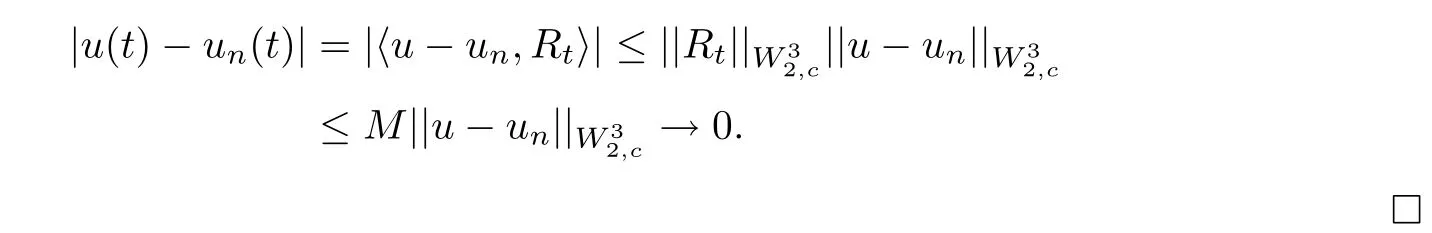
Similarly, we can prove that if t ∈[a,c]and[c,b]respectively,thenuniformly converges to u(i), i=1,2.

As N is continuous, and un→u uniformly, we have

Therefore, while u is the solution of Equation (6), and un=Pnu, we have

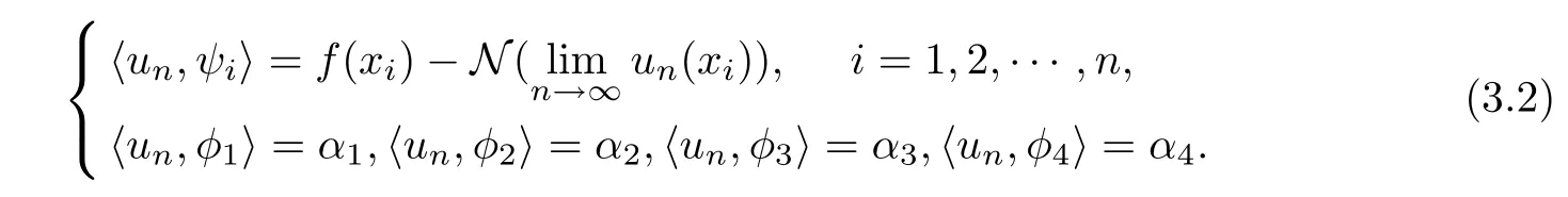
So, the approximate solution unof Equation (2.5) is the solution of Equation (3.3)

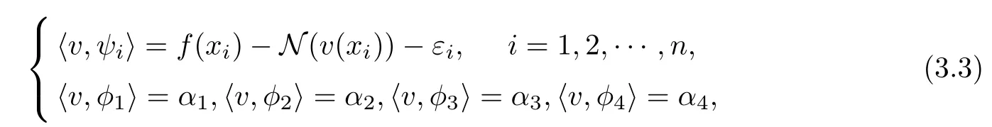
where εi=N(u(xi))−N(un(xi))→0 if n →∞.

As un∈Sn, so

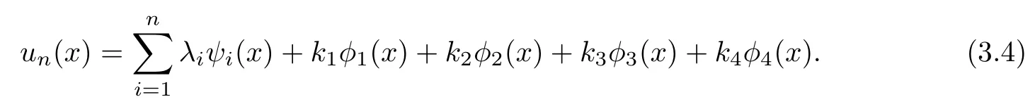
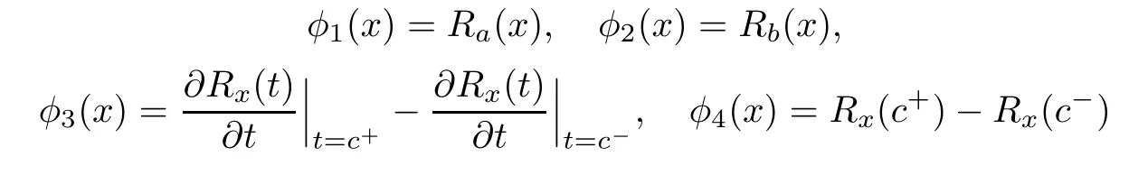
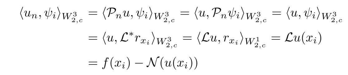
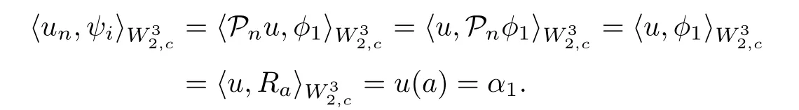
To obtain the approximate solution un, we only need to obtain the coefficients of each ψi(x) (i=1,2,··· ,n) and φj(x) (j =1,2,3,4). Use ψi(x) and φj(x) to do the inner products with both sides of Equation (3.4), we have

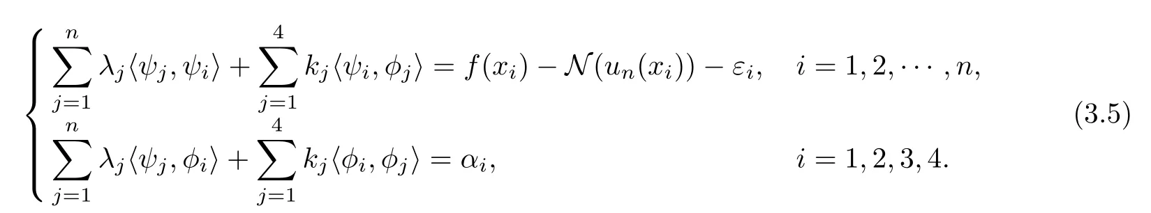
This is the system of linear equations of λi,kj,i=1,2,··· ,n, j =1,2,3,4.

Let

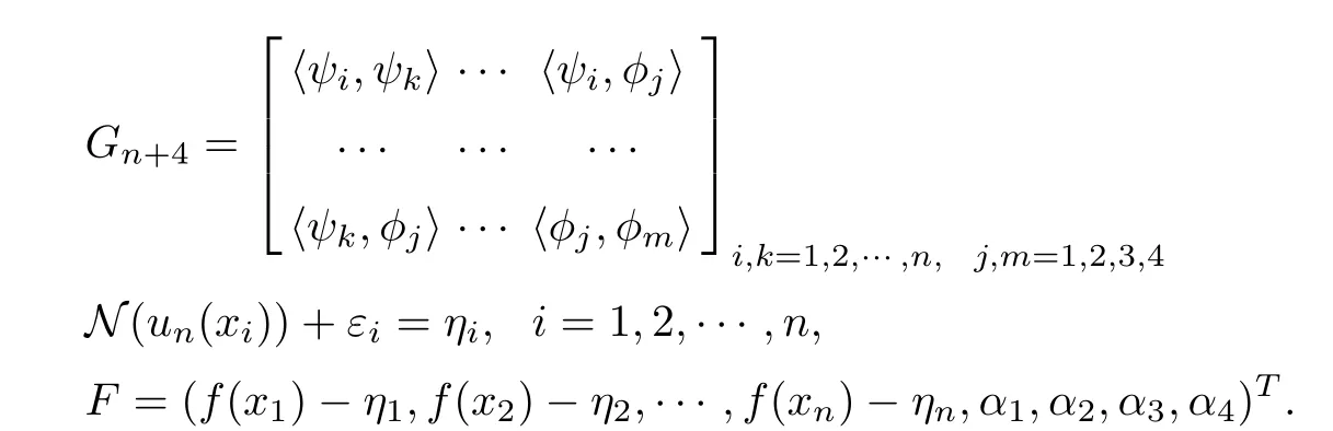
Then, we have

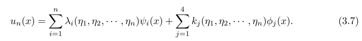
So, λ1,λ2,··· ,λn,k1,k2,k3,k4are expressed by η1,η2,··· ,ηn.

Substituting Equation (12) into Equation (3.4) yields

In order to solve the approximate solution unof Equation (2.5), it is necessary to make N(u(xi))and N(un(xi))close to the maximum,that is to say,each εiis as close as possible to 0.Therefore, we construct the following optimization model to solve the value of (η1,η2,··· ,ηn)

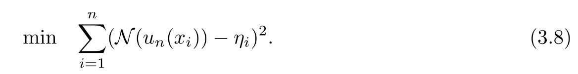
For the above model, it is actually a common nonlinear optimization problem, and there are many mature methods to solve the problem. In this article,the least square method is used to solve the minimum point () of Equation (3.8), and Mathematica software is used to implement the program, substituting (>) into Equation (3.7) to yield the solution unof Equation (3.4), namely, unis the approximate solution of Equation (2.5).

4 Numerical Examples

In this section, the method proposed in this article is applied to some impulsive differential equations to evaluate the approximate solution. In Examples 1–3, the reproducing space is[0,1]. Finally, the results show that our algorithm is practical and remarkably effective.

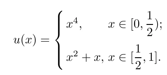
Example 4.1Consider the nonlinear impulsive differential equation:

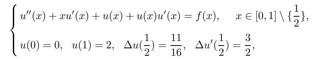
where

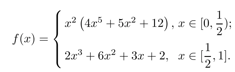
The exact solution

Example 4.2Consider the nonlinear impulsive differential equation:

where

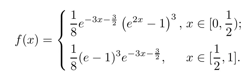
The exact solution

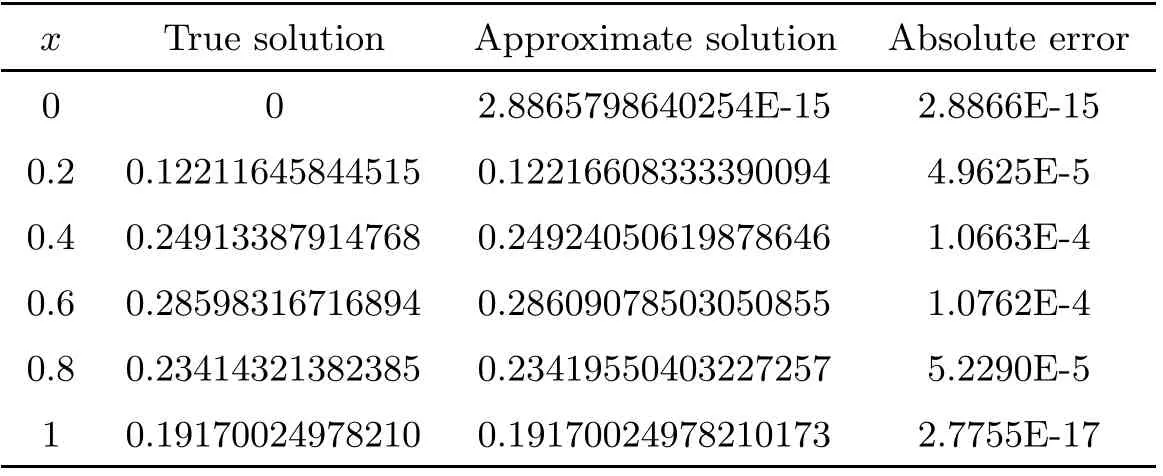
Table 2 Comparison of absolute errors in Example 2 (n=32)

In Figure 1 and Figure 2, the red dotted line is the numerical solution and the black line is the exact solution; it indicates that our presented method is very stable and effective. It is worth explaining that the method proposed in this article can not only be used to solve the nonlinear pulse problem, but also be used to solve the linear problems.

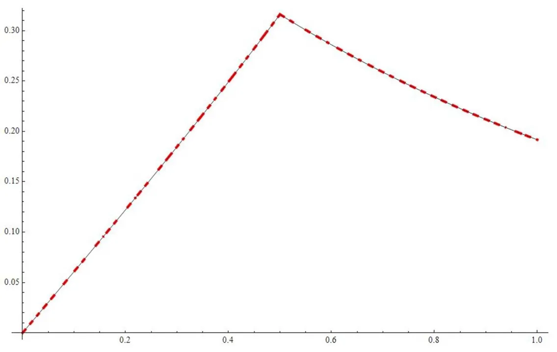
Figure 1 u and un in Example 2 (n=32)

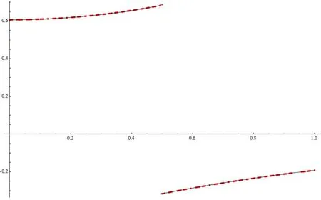
Figure 2 u′ and in Example 2 (n=32)

Example 4.3([14]) Consider the following impulsive differential equation with variable coefficients

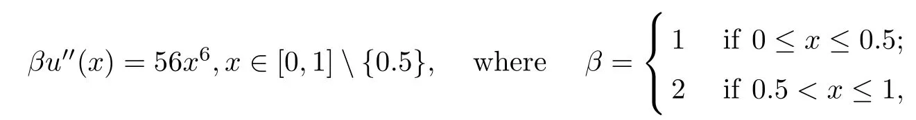
subject to the boundary and interface conditions:

The exact solution is

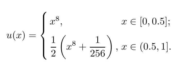
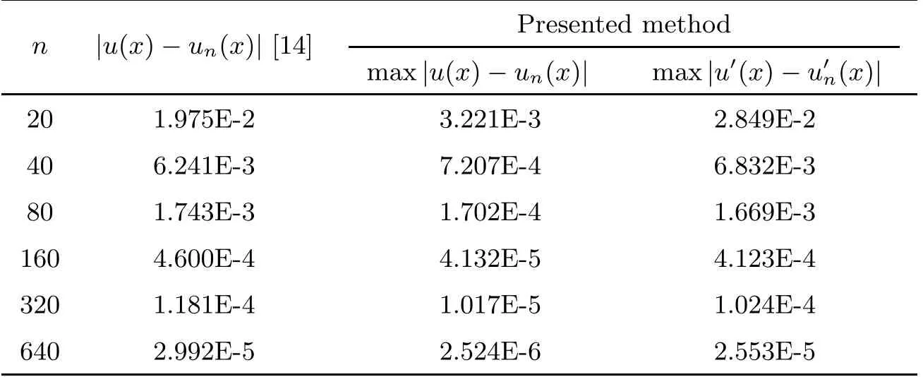
Table 3 Comparison of absolute errors in Example 3

5 Conclusion

In this article, combining the reproducing kernel method and the least square method to solve nonlinear impulsive differential equation, this method is proposed for the first time. A broken reproducing kernel space is cleverly built,and the reproducing kernel space is reasonably simple because the author did not consider the complicated boundary conditions, and avoid the time consuming Schmidt orthogonalization process. The nonlinear operator is transformed into a nonlinear optimization model, and the least square method is used to solve the problem.In fact, this technique can be extended to other class of impulsive boundary value problems.Although we just considered one pulse point in our presentation,by that analogy,the algorithm can also be applied to multiple pulse points. From the illustrative tables and figures, it is obtained that the algorithm is remarkably accurate and effective as expected.