Jie GU （顾杰）， Cheng-fei HU （胡成飞）， Cui-ping KUANG （匡翠萍）， Olaf KOLDITZ，Hai-bing SHAO （邵亥冰）， Jia-bo ZHANG （张甲波）， Hui-xin LIU （刘会欣）

1. College of Marine Sciences， Shanghai Ocean University， Shanghai 201306， China， E-mail: jgu@shou.edu.cn

2. Zhejiang Institute of Hydraulics and Estuary， Hangzhou 310020， China

3. College of Civil Engineering， Tongji University， Shanghai 200092， China

4. Helmholtz Centre for Environmental Research （UFZ）， Leipzig 04103， Germany

5. Qinhuangdao Mineral Resource and Hydrogeological Brigade， Qinhuangdao 066001， China

A water quality model applied for the rivers into the Qinhuangdao coastal water in the Bohai Sea， China*

Jie GU （顾杰）1， Cheng-fei HU （胡成飞）2， Cui-ping KUANG （匡翠萍）3， Olaf KOLDITZ4，Hai-bing SHAO （邵亥冰）4， Jia-bo ZHANG （张甲波）5， Hui-xin LIU （刘会欣）5

1. College of Marine Sciences， Shanghai Ocean University， Shanghai 201306， China， E-mail: jgu@shou.edu.cn

2. Zhejiang Institute of Hydraulics and Estuary， Hangzhou 310020， China

3. College of Civil Engineering， Tongji University， Shanghai 200092， China

4. Helmholtz Centre for Environmental Research （UFZ）， Leipzig 04103， Germany

5. Qinhuangdao Mineral Resource and Hydrogeological Brigade， Qinhuangdao 066001， China

The water quality of all rivers into the Qinhuangdao coastal water was below the grade V in 2013. In this study， an integrated MIKE 11 water quality model is applied to deal with the water environment in the rivers into the Qinhuangdao coastal water. The model is first calibrated with the field measured chemical oxygen demand （COD） concentrations. Then the transport of the COD in the rivers into the Qinhuangdao coastal water is computed based on the model in the water environmental monitoring process. Numerical results show that the COD concentration decreases dramatically in the estuaries， from which we can determine the positions of long-term monitoring stations to monitor the river pollutions into the coastal water. Furthermore， different scenarios about the inputs of the point sources and the non-point sources are simulated to discuss the model application in the water environmental control， and simplified formula are derived for assessing the water quality and the environmental management of rivers.

water environmental management， environmental monitoring and analysis， pollution control， water quality， MIKE 11，Qinhuangdao coastal wate

Introduction

The ocean is one of the most important natural resources in the economic development of coastal areas， related with， for instance， the ocean economy，including the coastal tourism， the marine communication， the transportation industry and the marine fishing industry， and it is now seen as a critical issue in China. The major ocean industries produced US$ 2.3909×1011in the value added output in 2010 and accounted for 4.03% of China's National Gross Domestic Product［1，2］. However， since the Industrial Revolution， in the global marine field， especially， in the coastal sea areas， the environments and the ecosystems become ever greater concerns due to the negative impacts of the urban effluent， the untreated effluent discharged into the sea，the agricultural runoff， the fishing and the shipping［3，4］. The agricultural， industrial， and municipal discharges are the main sources of pollutants released into the coastal marine environment through rivers［4］. The river pollutions， particularly those of the urban rivers， are one of the most serious water pollution issues of the present day［5，6］， which has great negative impacts on the quality of coastal waters. Thus， the water quality of the river into coastal waters should be taken into account in the water environmental management.

In water environmental management systems，there are various uncertainties that should be studied，such as the complicated hydrodynamic conditions， the process of the pollutant transport in the flow， and the degradation of the pollutant due to the biochemistryaction， etc.［7，8］. Among the accepted approaches to address these uncertainties are mathematical water quality models， to simulate the hydrodynamics and water quality transport processes［9，10］. In the last two decades， the most frequently used water quality models are QUAL2E［11］， Delft-3D［12］， WASP［13］and MIKE［14］. The selection of an appropriate numerical model mainly depends on the special objectives and the characteristics of the study area. The 2-D or 3-D models，for instance， are appropriate for studying the characteristics of the estuarine and coastal waters， but for a complicated catchment system， especially in case of requiring a long-term simulation， 1-D models are more appropriate［14，15］. MIKE 11 is a professional engineering software package for the simulation of flows，water quality and sediment transport in estuaries， rivers， irrigation systems， channels and other water bodies［16］.

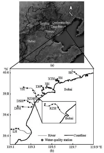
Fig.1 Geographical position of study area and water quality monitoring stations

Qinhuangdao is located in the northwest coast of the Bohai Sea and is well known as a famous summer resort （Fig.1（a））. It has a 162.7 km long coastline with many acclaimed bathing beaches for its soft fine sand and comfortable climate. However， in recent years， the increasing terrestrial pollutant emission into the Qinhuangdao coastal area has carried excess nutrients to the coastal waters， leading to red tide outbreaks frequently in the summer［17］. The frequently occurred extensive red tide blooms have significant negative impacts on the local bay scallop industry. It is found that about two thirds of the scallop cultivation area was affected by the blooms in 2009， and the bloom-affected area reached 3 350 km2in 2010， leading to an economic loss of RMB￥ 2×107［18］. To minimize the loss of red tide blooms， the State Oceanic Administration of China launched a Marine Public Welfare Program， including the emergency disposal of red tide outbreaks and the total emission control of pollutants in the Qinhuangdao coastal area. The total emission control of pollutants， especially， the control of river pollutant emission into the Qinhuangdao coastal water，can optimize the environment of the coastal water， and reduce the outbreak of red tides. However， since there are no long-term continuous monitoring stations in the estuaries of rivers into the Qinhuangdao coastal water，the control of water quality is difficult.

An integrated model for the water environmental management， including the environmental monitoring and the environmental control is proposed in this study. Based on MIKE 11， a water quality model is established to determine the chemical oxygen demand （COD）transport in the rivers. Then by using the water quality model， the simulation results in the water environmental monitoring and control， including ascertaining the positions of long-term monitoring stations and controlling point sources and non-point sources pollution，are discussed. Finally， some formulas are obtained for the environmental management of rivers based on the total quantity control plan and the governance costs of point sources.

1. Study area

Qinhuangdao （39o24＇N-40o37＇N， 118o33＇E-119o51＇E） is located in the northeast of Hebei Province， 280 km east of Beijing， China （Fig.1（a））， with an area of approximately 7 812 km2and a population of 2.9×106. Qinhuangdao enjoys a warm semi-humid continental monsoon climate， with mean annual temperature in the range of 9oC-11oC， the highest and the lowest monthly mean temperature in the range of 23oC-25oC and -7oC-5oC， respectively［19］. The nicest period in Qinhuangdao is from June to September （i.e.，the summer） for swimming in the sea.

There are ten primary rivers cross Qinhuangdao into the coastal water， which are， respectively， Shihe River （SH）， Tanghe River （TH）， Xiaotanghe River（XTH）， Xinhe River （XH）， Daihe River （DH）， Yanghe River （YH）， Renzaohe River （RZH）， Dongshahe River（DSH）， Dapuhe River （DPH）， and Luanhe River （LH）from north to south （Fig.1（a））. The study area extends 2.7 km-26.8 km in the upward river from each estuarine mouth， with the mean study river length of 11.9 km. The mean channel gradient and width of the ten rivers are 0.0692% and 147 m. Among these， the greatest and the least channel gradients are 0.1970%（SH） and 0.0031% （DSH）， respectively， and the widest and the narrowest rivers are LH of 369 m and XH of 47 m. The monthly runoff volumes （）W of ten rivers in 2013 are shown in Fig.2. The flood season （i.e.， the summer） of the rivers into the Qinhuangdao coastal water is from June to September， and the dry season is from November to February of the next year. It is found that LH， YH， DPH and TH have a larger runoff，with the maximum annual runoff of 1.3910×109m3in 2013 for LH， while XH has the minimum annual runoff， of just 4.5683×106m3. Because of drying-up in some rivers， the monthly mean runoff of TH and XTH is very small in the dry season.

Fig.2 Monthly runoff of 10 rivers in 2013

There are totally 54 water quality monitoring stations （Fig.1（b）） in the rivers into the Qinhuangdao coastal water. The monitoring time is August and November in 2013， which can be regarded as the representative months for the flood and dry seasons，respectively. Regularly monitored parameters include the COD， the total phosphorus （TP）， the ammonia nitrogen （NH4+-N） and the total nitrogen （TN）， which indicates that the water quality of all rivers is below the grade V in two seasons in 2013. The severest pollutant is the COD and its concentration is far higher than 40 mg/L （grade V standard value） in all rivers.

2. Methods

2.1Model description

The COD， a representative parameter widely used to estimate the organic content of wastewater［20］， is the severest in the ten rivers， with great negative impacts on the Qinhuangdao coastal water. For better management of the water environment of the Qinhuangdao coastal area， the river system in the Qinhuangdao coastal area is embedded into MIKE 11 for simulating the transport and analyzing the distribution of the COD in the rivers. MIKE 11， developed by DHI， is a userfriendly， fully dynamic， one-dimensional modelling tool for the detailed analysis， the design， the management and the operation of both simple and complex river systems. The hydrodynamic （HD） module is the core of the MIKE 11 modelling system and forms the basis for most modules including the Flood Forecasting， the advection-dispersion （AD）， the water quality and the sediment transport modules［16］.

The MIKE 11 HD module is used for computing the unsteady flow， the discharge and the water level in rivers and channels. It uses a one-dimensional， implicit， finite difference scheme for the numerical solution of the Saint-Venant equations and can be formulated as follows:

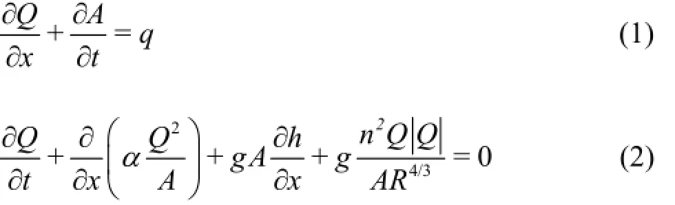
where Q is the discharge， x is the distance in the downstream direction， A is the cross section flow area， t is the time， q is the lateral inflow， g is the gravity acceleration， h is the water level above the reference datum， n is the Manning resistance coefficient， R is the hydraulic or resistance radius and α is the momentum distribution coefficient， introduced to account for the non-uniform vertical distribution of velocity in a given section［16］.

The computational grid is composed of alternating -Qpoints （discharge） and -hpoints （water level）along the river， with the -Qpoints being placed midway between adjacent -hpoints while the -hpoints being located on cross-sections［16］. The computational grid is automatically generated on the basis of themaximum distance， dx， defined as the distance between two adjacent -hpoints.

Fig.3 Comparison of computed and measured COD of 10 rivers in August， 2013

The water quality is computed by MIKE 11 AD module based on the advection-dispersion computation. The advection-dispersion computation uses a one-dimensional， implicit finite difference scheme for the numerical solution of the advection-dispersion equation， which is expressed as follows

where C is the concentration， D is the dispersion coefficient， K is the linear decay coefficient and 2C is the source/sink concentration［16］.

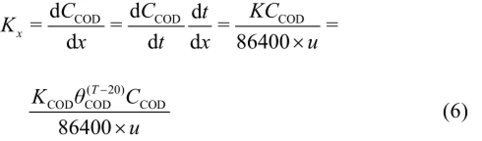
In this study， the COD is chosen as the representative index in the water quality model， and the CODtransport model based on Eq.（3） is established for the study of the COD variations. Normally， the COD concentration will decrease in the natural water， as in a degradation process， on account of microbial assimilation and metabolism. In this study， the COD degradation in the first-order decay process is adopted， as follows

Table 1 The positions of tidal current limits under typical hydrological conditions and suggested monitoring stations （m）

whereCODK is the degradation coefficient at 20oC， θCODis the Arrhenius temperature coefficient， and T is the water temperature.

2.2Model calibration

In the numerical model， the seaward open boundaries are driven by the tidal level and the COD concentration provided by our well calibrated COD transport model in the whole Qinhuangdao coastal area. The upstream boundaries are driven by the monthly measured runoff and the COD concentration. The Manning resistance coefficients （）n are specified as in the range of 0.02 s/m1/3-0.05 s/m1/3according to the distribution of the measured sediment size and water depth. The dispersion coefficients （）D， the COD decay coefficient at 20oCCOD（）K and the Arrhenius temperature coefficientCOD（）θ are calibrated by the COD transport model， setting as 10 m2/s-100 m2/s，0.05 d-1-0.4 d-1and 1.02， respectively. The COD initial concentration0（）C is specified as in the range of 56 mg/L-84 mg/L， in accordance with the COD mean concentration of the rivers in June. The computation period is from June 1 to November 30， 2013， and the time step is 40 s.

These parameters are calibrated on the basis of the measured data in August， 2013， and the comparison of computed and measured COD concentrations of each river is shown in Fig.3. The -xaxis represents distance from each estuary （=0）D toward the upstream. The computed COD concentrations along ten rivers are in a good agreement with the measured values.

Generally， the model performance can be evaluated on the basis of the qualitative method， the percent bias （PBIAS） is selected to quantitatively evaluate the model. The PBIAS is given by

where M is the measured value， C is the computed value， N is the total number of measured data. For pollutants， the predictive efficiency of a model is classified as very good for PBIAS less than 25， good for PBIAS in the range of 25-40， satisfactory for PBIAS in the range of 40-70， and unsatisfactory for PBIAS larger than 70［21］.

The computed PBIAS values for all stations are between 0.9-10.6， which implies that the model is very good in the predictive efficiency. Thus， this model is acceptable with a reliable performance in simulating the COD in the rivers into the Qinhuangdao coastal water.

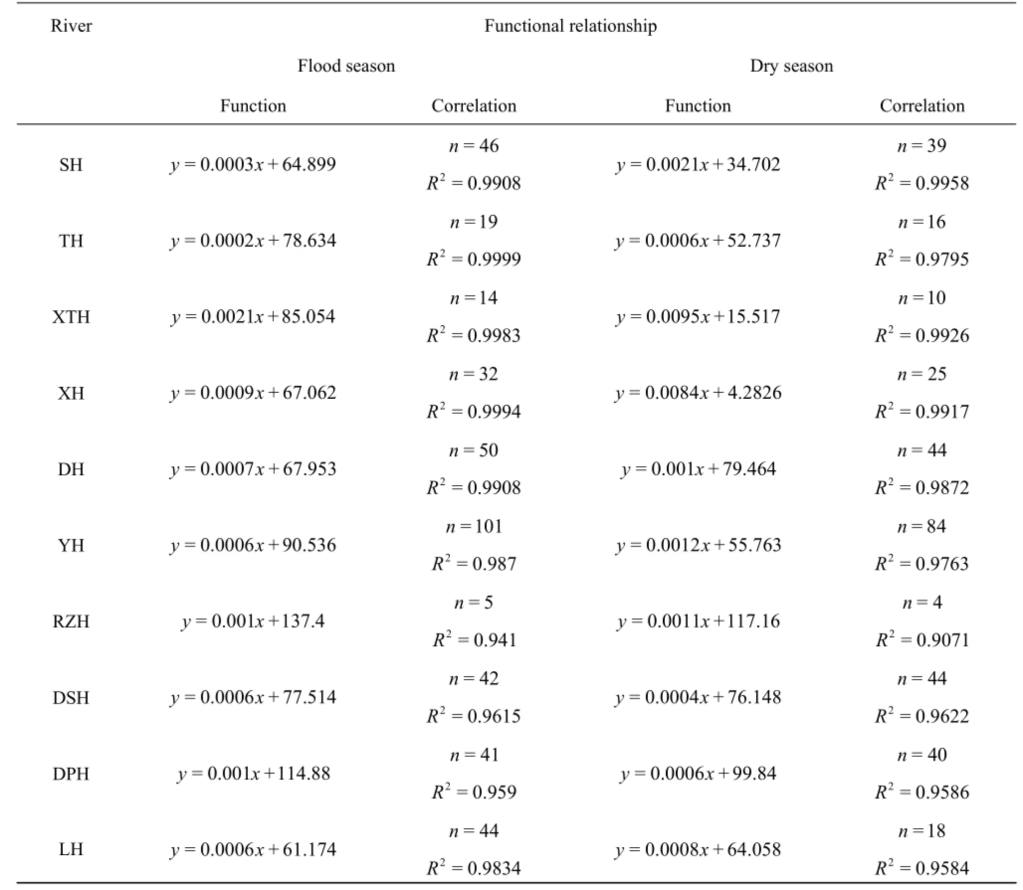
Table 2 The functional relationships between COD concentration and distance from estuary in the upstream of tidal current limit

3. Results and discussions

3.1Application in water environmental monitoring

The water environmental monitoring is the basis of the water environmental management， especially for estuarine waters. It is crucial to monitor the terrestrial pollutants through the influx of the river into the coastal water. However， there are no fixed long-term stations to monitor the hydrology and the water quality consecutively in the rivers into the Qinhuangdao coastal water. To set up a monitoring station to obtain long-term observations， the position of the monitoring station is one of the decisive factors as far as the monitoring accuracy of the terrestrial pollutants into coastal waters is concerned， which means that the position must be in the upstream of the tidal current limit where there is the maximum flood current. Otherwise，the measured concentration of the terrestrial pollutants will be affected due to the large amount of the tidal current mixing， with additional dilution and the measured concentration will be much lower than that in the fresh river water. Figure 3 indicates that the COD concentration decreases slightly in the upstream of the rivers due to the mixing and dilution of the runoff， the microbial assimilation and the metabolism. However，it decreases dramatically in the estuary because of the tidal mixing and high dilution. Thus， the tidal current limit can be derived through the COD concentration sudden variation along the rivers. In this study， on a certain river cross section， if the longitudinal gradient of the COD concentration in its downstream is over twice of that in its upstream， this cross section can betaken as in the vicinity of the tidal current limit. For example， for a cross section at x=1418 in DH， the longitudinal gradient of the COD concentration in DH（Fig.3） is 0.124% in its downstream， whereas it is 0.059% in its upstream， therefore the cross section from the estuary （x=0） of DH with a length of 1 418 m can be determined as the tidal current limit for DH.

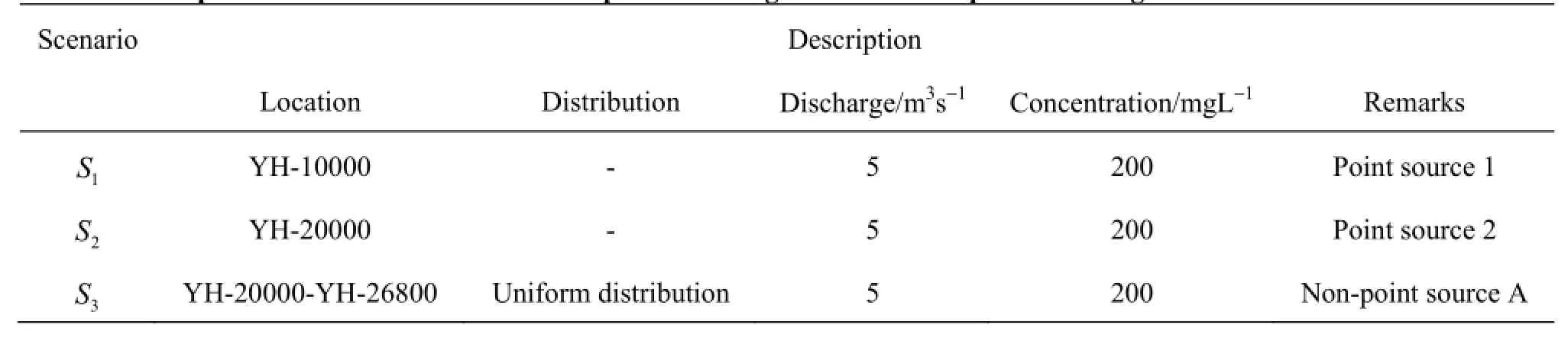
Table 3 Description of three scenarios with two point discharges and one non-point discharge

The positions of the tidal current limit for each river under typical hydrological conditions are shown in Table 1. The distance between the tidal current limit and the corresponding estuary is found to be largely determined by the interaction of the river runoff and the ocean tides， i.e.， the distance has a negative correlation with the river runoff and a positive correlation with the tidal range. It is prerequisite for the estuarine and coastal water environment management to set up monitoring stations that can monitor the hydrology and the water quality continuously. The computed positions of the tidal current limit for ten rivers are based on the hydrologic conditions of Qinhuangdao in 2013， for safety and uncertainty reasons， the monitoring station at the position of 1.1 times of the distance of the tidal current limit from the estuary is proposed，and the corresponding suggested monitoring stations for ten rivers are listed in Table 1.

3.2Application in water environmental contorl

The water environmental control is the main task of the water environmental management. In the estuarine and coastal area， it is imperative to control the pollutant influx into coastal waters. The distributions of the COD concentration along the rivers shown in Fig.3 show that the relationship between the COD concentration and the distance from the estuary can be well fitted by a linear function in the upstream of the tidal current limit， i.e. there is a similar attenuation ratio along the river in the upstream of the tidal current limit. The functional relationships between the COD concentration and the distance from the estuary in the upstream of the tidal current limit are given in Table 2. If the COD concentration at the YH tidal current limit is required to be less than 60 mg/L in the flood season，for instance， the COD concentration should be controlled to be less than 66 mg/L at 10 km in the upstream of the tidal current limit.

With Eq.（4）， i.e.， the COD degradation process equation， the COD attenuation ratio along the river can be expressed as follows

wherexK is the COD attenuation ratio along the river， CCODis the COD concentration， and u is the flow velocity. Hence， the COD attenuation ratio along the river is not only determined by the water temperature（）T and the decay coefficient at 20oCCOD（）K， but also affected by the river runoff （i.e.， the river flow velocity）.

The water environment control involves the controls of the point sources and the non-point sources and the management［5，22］. In order to better control the water environment， the influences of the point sources or the non-point sources can be pre-evaluated through the water quality model. The industries of the agriculture and the processing of the agricultural by-products are assembled in the YH drainage basin， and they carry pollutions of some non-point sources and point sources into YH. To evaluate the influence of the point sources and the non-point sources on YH， other three scenarios are designed as listed in Table 3 and the results are compared with those of the present scenario called as0S.

The computed daily mean concentrations of the COD along YH in three scenarios1S，2S and3S based on the numerical model are compared with the present scenario0S and shown in Fig.4. It can be seen that the COD has already been fully mixed at the tidal current limit in all scenarios， andxK in all scenarios takes a similar value. The supposed point sources in scenarios1S and2S are1x and2x away from the tidal current limit， the concentration of the COD at the tidal current limit in scenarios1S and2S can bederived as follows:

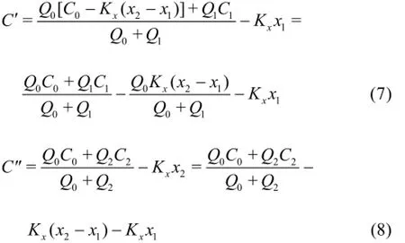
where C＇ and C＇ are the COD concentrations at the tidal current limit in scenarios1S and2S， respectively， Q0and C0are the flow discharge and the COD concentration at YH-20000 in scenario S0， respectively， Q1and Q2are the point source discharge in scenarios S1and S2， respectively； C1and C2are the COD concentrations of the point source in scenarios S1and S2， respectively.

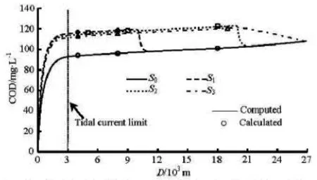
Fig.4 Comparison of computed （from numerical model） and calculated （from Eqs.（6）-（8）） daily mean concentrations of COD along YH under four scenarios

The COD daily mean concentrations in all scenarios can be calculated by Eqs.（6）-（8）， and the results shown in Fig.4 indicate a good agreement with the computed values using the numerical model， i.e.， the water quality in the rivers can be well assessed using these equations. In this study，12=QQ，12=CC， thus， C＇＞C＇＇， that means that， for the same point source， the nearer the point source from the estuary， the greater the increase of the pollutant concentration into the coastal water will be. The non-point source A is uniformly distributed on x2-x3， and its mathematical expectation is （x2+x3）/2， i.e.， the non-point source A is equivalent to a point source on （x2+x3）/2. Thus， the order of the high COD concentrations into the coastal water in all scenarios is S1＞S2＞S3.

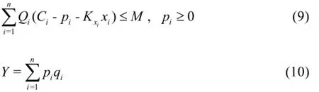
As expected， the point source released in the upstream of the tidal current limit will not affect its upstream due to the fact that the river in this region assumes a single downward flow. Therefore the total quantity control plan and governance costs of point sources can be evaluated as follows: where M is the total quantity control objective at the control section，iQ andiC are the flow discharge and the pollutant concentration of the thi point source，respectively，ip is the reduced pollutant concentration quantity of the thi point source，ixK is the pollutant attenuation ratio along the river of the thi point source， which can be obtained from Eq.（6） or the water quality numerical model，ixis the distance between the thi point source and the control section， Y is the total cost of the point source control，iq is the unit governance cost of the thi point source.

Combining the pollution analysis with the governance costs of each point source in the drainage basin，the optimal plan for the point sources control can be obtained using the linear programming method， i.e.，the total quantity control objective of the control section （Eq.（9）） under the lowermost governance costs（the minimum Y in Eq.（10））. The non-point source is equivalent to various point sources with different regularities of pollutant distribution， and the optimal pollution control plan can be obtained through Eqs.（9）-（10）.

4. Conclusions

An integrated MIKE 11 water quality model system， comprising of a hydrodynamic model （MIKE 11 HD） and a water quality model （MIKE 11 AD）， is successfully calibrated and applied to manage the water environment in the rivers into the Qinhuangdao coastal water.

The COD concentration decreases slightly in the upstream of the river， but decreases dramatically in the estuary because of tidal mixing and high dilution. This feature is used to determine the positions of the tidal current limit based on numerical simulations of the COD transport in different seasons and for different tides. The distance between the tidal current limit and the corresponding estuary is largely determined by the interaction of the river runoff and the oceantides， and has a negative correlation with the river runoff and a positive correlation with the tidal range. Further， the positions of the long-term monitoring stations to monitor the river pollutions into the coastal water for the ten rivers are suggested.

Different scenarios about the inputs of the point sources and the non-point sources are simulated in the model application for the water environmental control，and it is concluded that the COD attenuation ratio along the river is determined by the COD degradation process and the river runoff. The effect of the pollution sources on coastal waters is in a negative correlation with the distance between the pollution source and the estuary， thus it is imperative to reduce the COD concentration into coastal waters in order to control the pollution source input. The optimal solution to the control point sources is obtained by using the linear programming method based on combining the pollution analysis with the governance costs of each point source in the drainage basin. In conclusion， the water quality model can be used as an effective tool to evaluate the effects of the pollution sources and study the transport of the pollutants， and it can be well applied in the water environmental management.

References

［1］ZHAO R.， HYNES S. and HE G. S. Defining and quantifying China's ocean economy［J］. Marine Policy， 2014， 43: 164-173.

［2］MORRISSEY K. Using secondary data to examine economic trends in a subset of sectors in the English marine economy: 2003-2011［J］. Marine Policy， 2014， 50（3）: 135-141.

［3］ISLAM M. S.， TANAKA M. Impacts of pollution on coastal and marine ecosystems including coastal and marine fisheries and approach for management: a review and synthesis［J］. Marine Pollution Bulletin， 2004， 48（7-8）: 624-649.

［4］LI K.， SHI X. and BAO X. et al. Modeling total maximum allocated loads for heavy metals in Jinzhou Bay， China［J］. Marine Pollution Bulletin， 2014， 85（2）: 659-664.

［5］SCHAFFNER M.， BADER H. and SCHEIDEGGER R. Modeling the contribution of point sources and non-point sources to Thachin River water pollution［J］. Science of the Total Environment， 2009， 407（17）: 4902-4915.

［6］XUE Chong-hua， YIN Hai-long and XIE Ming. Development of integrated catchment and water quality model for urban rivers［J］. Journal of Hydrodynamics， 2015， 27（4）: 593-603.

［7］LI Y. P.， HUANG G. H. Two-stage planning for sustainable water-quality management under uncertainty［J］. Journal of Environmental Management， 2009， 90（8）: 2402-2413.

［8］XIE Y. L.， LI Y. P. and HUANG G. H. et al. An inexact chance-constrained programming model for water quality management in Binhai New Area of Tianjin， China［J］. Science of the Total Environment， 2011， 409（10）: 1757-1773.

［9］RAUCH W.， HENZE M. and KONCSOS L. et al. River water quality modelling: I. State of the art［J］. Water Science and Technology， 1998， 38（11）: 237-244.

［10］ COX B. A. A review of currently available in-stream water-quality models and their applicability for simulating dissolved oxygen in lowland rivers［J］. Science of the Total Environment， 2003， 314-316: 335-377.

［11］ PALIWAL R.， SHARMA P. and KANSAL A. Water quality modelling of the river Yamuna （India） using QUAL2E-UNCAS［J］. Journal of Environmental Management， 2007， 83（2）: 131-144.

［12］ CHEN Q.， WU W. and BLANCKAERT K. et al. Optimization of water quality monitoring network in a large river by combining measurements， a numerical model and matter-element analyses［J］. Journal of Environmental Management， 2012， 110: 116-124.

［13］ ZHANG Ming-liang， SHEN Yong-ming and GUO Ya-kun. Development and application of a eutrophication water quality model for river networks［J］. Journal of Hydrodynamics， 2008， 20（6）: 719-726.

［14］ CHIBOLE O. K. Modeling River Sosiani's water quality to assess human impact on water resources at the catchment scale［J］. Ecohydrology and Hydrobiology， 2013，13（4）: 241-245.

［15］ ZHOU N. Q.， WESTRICH B. and JIANG S. M. et al. A coupling simulation based on a hydrodynamics and water quality model of the Pearl River Delta， China［J］. Journal of Hydrology， 2011， 396（3-4）: 267-276.

［16］ HU Lin， LU Wei and ZHANG Zheng-kang. Application of MIKE11 model in water quality early-warning and protection in Dong Tiaoxi water source［J］. Chinese Journal of Hydrodynamics， 2016， 31（1）: 28-36（in Chinese）.

［17］ LIU S.， LOU S. and KUANG C. et al. Water quality assessment by pollution-index method in the coastal waters of Hebei Province in western Bohai Sea， China［J］. Marine Pollution Bulletin， 2011， 62（10）: 2220-2229.

［18］ ZHANG Q. C.， QIU L. M. and YU R. C. et al. Emergence of brown tides caused by Aureococcus anophagefferens Hargraves et Sieburth in China［J］. Harmful Algae， 2012，19: 117-124.

［19］ WANG Su-lan， WANG Li-ying. Development tentative plan of Beidaihe scenic spot in Qinhuangdao［J］. Journal of Tongji University： Social Science Section， 1994（S1）: 40-43（in Chinese）.

［20］ VYRIDES I.， STUCKEY D. C. A modified method for the determination of chemical oxygen demand （COD） for samples with high salinity and low organics［J］. Bioresource Technology， 2009， 100（2）: 979-982.

［21］ MORIASI D. N.， ARNOLD J. G. and Van LIEW M. W. et al. Model evaluation guidelines for systematic quantification of accuracy in watershed simulations［J］. Transactions of the Asabe， 2007， 50（3）: 885-900.

［22］ LAI Y. C.， YANG C. P. and HSIEH C. Y. et al. Evaluation of non-point source pollution and river water quality using a multimedia two-model system［J］. Journal of Hydrology， 2011， 409（3-4）: 583-595.

（May 30， 2016， Revised June 28， 2016）

* Project supported by the Marine Public Welfare Program of China （Grant No. 201305003-5） and the Science and Technology Program of the Oceanic Administration of Hebei Province of China.

Biography： Jie GU （1961-）， Male， Ph. D.， Professor

Cui-ping KUANG，

E-mail: cpkuang@tongji.edu.cn