GONG Jian-wei(龚建伟), XU Wei(徐威), JIANG Yan(姜岩), LIU Kai(刘凯), GUO Hong-fen(郭红芬), SUN Yin-jian(孙银健)

(School of Mechanical Engineering, Beijing Institute of Technology, Beijing 100081, China)



Multi-constrained model predictive control for autonomous ground vehicle trajectory tracking

GONG Jian-wei(龚建伟), XU Wei(徐威), JIANG Yan(姜岩), LIU Kai(刘凯), GUO Hong-fen(郭红芬), SUN Yin-jian(孙银健)

(School of Mechanical Engineering, Beijing Institute of Technology, Beijing 100081, China)

A multi-constrained model predictive control (MPC) algorithm for trajectory tracking of an autonomous ground vehicle is proposed and tested in this paper. First, to simplify the computation, an active steering linear error model is applied in the MPC controller. Then, a control increment constraint and a relaxing factor are taken into account in the objective function to ensure the smoothness of the trajectory, using a softening constraints technique. In addition, the controller can obtain optimal control sequences which satisfy both the actual kinematic constraints and the actuator constraints. The circular trajectory tracking performance of the proposed method is compared with that of another MPC controller. To verify the trajectory tracking capabilities of the designed controller at different desired speed, the simulation experiments are carried out at the speed of 3m/s, 5m/s and 10m/s. The results demonstrate the MPC controller has a good speed adaptability.

autonomous ground vehicle; active steering control; model predictive control; trajectory tracking

Active steering techniques play a very important role in a fully autonomous ground vehicle (AGV) control system[1]. Trajectory tracking control is one of the basic control problems in active steering. It requires the AGV to reach a given or planned point at a specified time. Since a ground vehicle is a strongly nonlinear and highly coupled system, the trajectory tracking control of the AGV has always been a difficulty. Many methods and techniques have been proposed for trajectory tracking of the AGV, including backstepping[2-3], dynamic feedback linearization[4], sliding mode control[5], etc. Some intelligent control methods, such as fuzzy control[6], neural network control[7], and rolling optimization control[8], have also been gradually applied in this research and engineering practice. However, most of these methods regard a vehicle as a mobile robot, not further considering various constraints of the vehicle in the process of trajectory tracking. With limited constraints of the steering control quantity and smoothness constraints of the control increment, the vehicle cannot follow the control quantity in every control cycle. This will lead to the jitter phenomenon in trajectory tracking.

Model predictive control (MPC) method, which combines predictive models, a receding horizon optimization and a feedback correction, has a very good ability to solve the control problem with multiple constraints. The constraints are used to build the objective function of an MPC controller to obtain an optimal control output. According to the difference of prediction models, the MPC can be divided into nonlinear MPC and linear MPC[9]. Although the nonlinear MPC has been well developed, its computation consumption is much higher than that of the linear MPC controller[10]. As the constraint proposed in Ref. [10] has no experimental verification, it cannot ensure the control output is carried out before the next control cycle. A trajectory tracking method based on the linear MPC is proposed in Ref.[11], in which the vehicle steering constraints are taken into consideration. However, it does not consider constraints of the control increment in the objective function. As a result, an abrupt change of the control quantity is inevitable.

In this paper,we try to take as many constraints as possible into consideration when constructing the MPC objective function. Compared with the previous work, the following improvements can be achieved. First, to ensure the smoothness of the control quantity and the vehicle’s maneuver, a control increment constraint and a relaxing factor are added into the objective function. Second, we obtain the optimal control sequences to the actual kinematic constraints and actuator constraints of the vehicle, which result from the longitudinal and lateral tracking simulation and real vehicle tests. Also, to some extent, dynamic characteristics of the AGV in actual movement are considered. Finally, the comparative experiments of the circular trajectory tracking capability of two different controllers are implemented in the CarSim/Simulink platform.

1 Vehicle kinematic modeling

The simplified front-wheel steering vehicle kinematic model is shown in Fig. 1. In the global coordinate systemXOY, the vehicle kinematic equation can be expressed as

(1)

where (x,y) is the coordinate of the rear axle center,θis the heading angle of the vehicle body,δis the front wheel angle,vis the speed of the rear axle, andlis the wheel base.

Fig.1 Vehicle kinematic model

In Eq.(1), the system can be viewed as a control system with an input u(v,δ) and a state variableχ(x,y,θ). The general form is

(2)

Assuming that each point on the given reference trajectory satisfies the kinematic equation above, the general form can be expressed as

(3)

whereχr=[xryrθr]T, ur=[vrδr]T.

Using the Taylor series expansion at the reference trajectory point in Eq.(2) and ignoring higher order terms, we can obtain

(4)

Subtracting Eq.(3) from Eq.(4) results in

(5)

Eq.(5) is the linear error model of the AGV. In order to apply the model to the design of the MPC controller, Eq.(5) can be discretized as

(6)

2 Model predictive controller

The design concept of the MPC controller is to convert an actual control problem into an objective function with constraints. Optimizing the objective function, we can obtain the control sequences in a future horizon section. Then the first of them is applied to the control system. The MPC controller is designed based on the linear error model. The objective function is linearized and converted into a quadratic program (QP), which can be easier to calculate.

The algorithm diagram of the trajectory tracking controller is shown in Fig.2, where the dashed box represents the MPC controller mainly composed of the linear error model, system constraints, and the objective function. Since the linear error model of the AGV has been identified, the main content of the controller design is to construct an appropriate objective function, which can combine the constraints of AGV’s active steering system.

Fig.2 Trajectory tracking MPC controller

2.1 Objective function

The ability of the objective function is to make the AGV track the desired trajectory rapidly and smoothly. Therefore, the system status deviation and the optimization of the control output should be combined into the controller. The objective function of the trajectory tracking controller in Ref.[11] is

(7)

where Q and R represent weight matrices. The first term in Eq.(7) reflects the capability of the system to track the reference trajectory, while the second reflects the constraint on the change of the control output. The advantage of the above objective function is that it can be easily converted into the standard form of quadratic programming, but there are obvious flaws:the control increment in each sampling period cannot be limited. In other words, the phenomenon of the control output mutation cannot be avoided, and thus the continuity of the control output cannot be ensured. Referencing to the soft constraints concept in Ref. [12], we can get the following objective function:

(8)

whereNpis the predictive horizon,Ncis the control horizon,ρis the weight coefficient, andεis the relaxing factor.

Compared with Eq.(7), Eq.(8) adds a relaxing factor and has the control increment instead of the control output. This will not only allow for a direct limiting of the control increment, but will also prevent emerging infeasible solutions during execution.

In the objective function, the control output of the system in a section of the future horizon can be predicted using the linear error model of the AGV. And Eq. (6) can be converted to

(9)

A new expression of the state space is obtained as

(10)

Also, the following hypothesis is made to simplify the calculation as

Ak,t=At,t,k=1,…,t+N-1 Bk,t=Bt,t,k=1,…,t+N-1

(11)

As a result, the following predicted output expression of the system can be obtained after deduction:

Y(t)=Ψtξ(t|t)+ΘtΔU(t)

(12)

where

Substituting Eq. (12) into Eq. (8) can result in the complete form of the objective function.

2.2 Constraints description

The limiting constraints of the control output quantity and the control increment constraints in the trajectory tracking control will be considered as the main factors in our work. The control output quantity can be expressed as

umin(t+k)≤u(t+k)≤umax(t+k),k=0,1,…,Nc-1

(13)

And the expression of the control increment constraint is

Δumin(t+k)≤Δu(t+k)≤

Δumax(t+k),k=0,1,…,Nc-1

(14)

In the objective function,the variables to be solved are control increments in the control horizon. The constraint conditions can only be expressed as a form of the control increment or a form of the control increment multiplied by the transformation matrix. Thus, Eq.(14) needs to be converted for obtaining the corresponding transformation matrix. The relationship is defined as

u(t+k)=u(t+k-1)+Δu(t+k)

(15)

We assume that

Ut=1Nc⊗u(k-1)

(16)

(17)

where 1Ncis the column vector ofNcones, Imis the identity matrix with a dimension ofm, ⊗ is Kronecker product, and u(k-1) is the previous control input.

Combining Eqs.(15)(16)(17), Eq.(13) can be converted into

Umin≤AΔUt+Ut≤Umax

(18)

where Uminand Umaxare the lower and upper bounds of the control input, respectively.

To solve the following optimization problem,the objective function is converted into a standard quadratic form with one constraint condition.

J(ξ(t),u(t-1),ΔU(t))=[ΔU(t)T,ε]THt[ΔU(t)T,ε]+Gt[ΔU(t)T,ε]

(19)

s.t.ΔUmin≤ΔUt≤ΔUmaxUmin≤AΔUt+Ut≤Umax

After obtaining the solution to Eq.(19) in each control cycle, a series of control input increments in the control horizon can be calculated as

(20)

The first element of the control sequences is taken as the actual control input increment of the controller.

(21)

The above process is repeated continuously in every control cycle, and the AGV can track the desired trajectory.

3 Simulation experiment

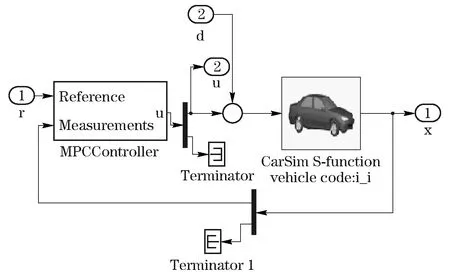
Fig.3 Co-simulation platform of CarSim/Simulink

In order to verify the performance of the MPC based trajectory tracking controller, a co-simulation CarSim/Simulink platform, which is composed of the CarSim module and the trajectory tracking controller module, is built in this work (Fig.3). In the simulation platform, the trajectory tracking controller module is structured by a Simulink S-function. The sampling frequencies of CarSim and the trajectory tracking controller are set to 1 000 Hz and 20 Hz, respectively.

Vehicle motion parameters in the actual system are determined by a road input and vehicle suspension characteristics. However, the vehicle motion parameters on the simulation platform are calculated by the built-in road model and the multi-rigid-body dynamics model of CarSim[13-14]. The CarSim module receives the control output quantity of the trajectory tracking controller and outputs the real-time vehicle motion parameters, including the global coordinates of the vehicle location, the heading angle and the longitudinal and lateral speed. The trajectory tracking controller receives a reference trajectory input and a measuring input, then outputs the control quantity, including the front-wheel steering angle and the longitudinal speed. The control output quantity of the actuator is implemented by the built-in controller of CarSim.

3.1 Tracking capability tests

In order to make the controller constraints reflect the actual constraints of the AGV, the longitudinal and lateral tracking capability of a real AGV testbed is tested. We take the AGV testbed in Refs.[1] [15] as a prototype of this work.

In the longitudinal tracking experiment, three expected vehicle step speeds, 5 m/s, 7.5 m/s and 10 m/s, are set to test step speed response characteristics. After the vehicle running at each speed for several minutes, the maximum brake force is applied to the vehicle to test the deceleration performance. The corresponding acceleration and deceleration times are listed in Tab.1. The vehicle is relatively smooth when accelerating and decelerating within the middle-low speed range (7.5 m/s or less) and its acceleration remains at about 1 m/s2. To make the tracking process more stable, the vehicle speed deviationveconstraint and the speed increment in every control cycle Δvconstraint can be set to

-0.2 m/s≤ve≤0.2 m/s-0.05 m/s≤Δv≤0.05 m/s

(22)

Tab.1 Test of the longitudinal tracking capability of the AGV testbed

speed/(m·s-1)accelerationtimetj/sbrakingtimetz/s0-5560-7 5880-101512

In the lateral tracking test, the front wheels are steered continuously from the left limiting position to the right limiting position. The corresponding position and elapsed time are listed in Tab. 2. It takes about 1.8 s to turn the steering wheel for a circle, corresponding to the front-wheel steering angle of about 17 °.

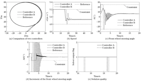
Fig.4 Comparison of the trajectory tracking capability of two controllers

Tab.2 Test of the lateral steering actuator’s performance

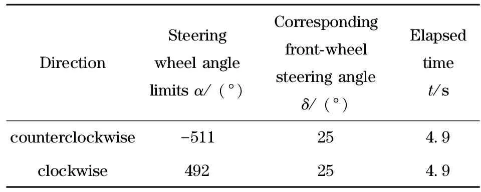
DirectionSteeringwheelanglelimitsα/(°)Correspondingfront⁃wheelsteeringangleδ/(°)Elapsedtimet/scounterclockwise-511254 9clockwise492254 9

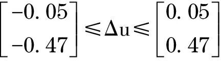
Therefore, the limitation and the increment of the front-wheel steering angle can be set to

-25°≤δ≤25°-0.47°≤Δδ≤0.47°

(23)

Combining Eq.(22) and Eq.(23), we can obtain the control output quantityuconstraint and the control increment Δu constraint.

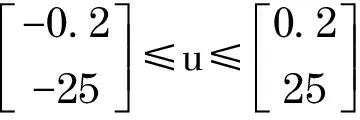
(24)

(25)

3.2 Results of trajectory tracking simulation tests

We design a set of tests to compare the trajectory tracking performance between our proposed method (controller A, in Eq. (8)) and the method illustrated in Ref.[11] (controller B, in Eq. (7)). The objective functions in controller A and B are designed with methods of soft constraints and hard constraints, respectively.

The results in Fig. 4a show that the circular reference trajectory can be tracked quickly by both the controller A and B when there is an initial deviation between the AGV and the circular reference trajectory. In Fig. 4b and Fig. 4c, we can see that there is the “jitter” phenomenon for a long time in the control output quantity curve of controller B, however, the control output quantity of controller A is always smooth. Furthermore, Fig.4d demonstrates that as there is no constraint on the control increment of controller B, the control increment changes sharply, and it cannot be executed by the actuator. However, the control increment of controller A is always limited by the constraint. In Fig. 4e, the solver output flag is reported. In our tests, the value 0 indicates that the limit on the iteration number has been reached, but the optimal solution hasn’t been found. The value 1 is returned when an optimal feasible solution is found. We can see that controller B does not find the optimal solution occasionally. Thus, by adding the control increment constraint and the relaxing factor in the objective function, it is possible to significantly reduce the “jitter” phenomenon and ensure the smoothness of the control output quantity.

Speed adaptability is a very important characteristic of a trajectory tracking controller. Fig. 5 shows the tracking results of the controller A when the AGV runs at the speed of 3 m/s, 5 m/s, and 10 m/s, respectively. Fig. 5a shows that the AGV can follow the desired trajectory, and the position error goes to zero quickly, as shown in Fig. 5b. The time used to follow the circular trajectory is 52.10 s, 31.75 s, and 15.75 s, respectively. We can see that the control algorithm has a good convergence. Fig. 5c and Fig.5d show that the control output quantity and the control increment of the MPC controller are all limited in the constraint horizon and have no abrupt changes. So, we can conclude that the MPC controller has a good speed adaptability.

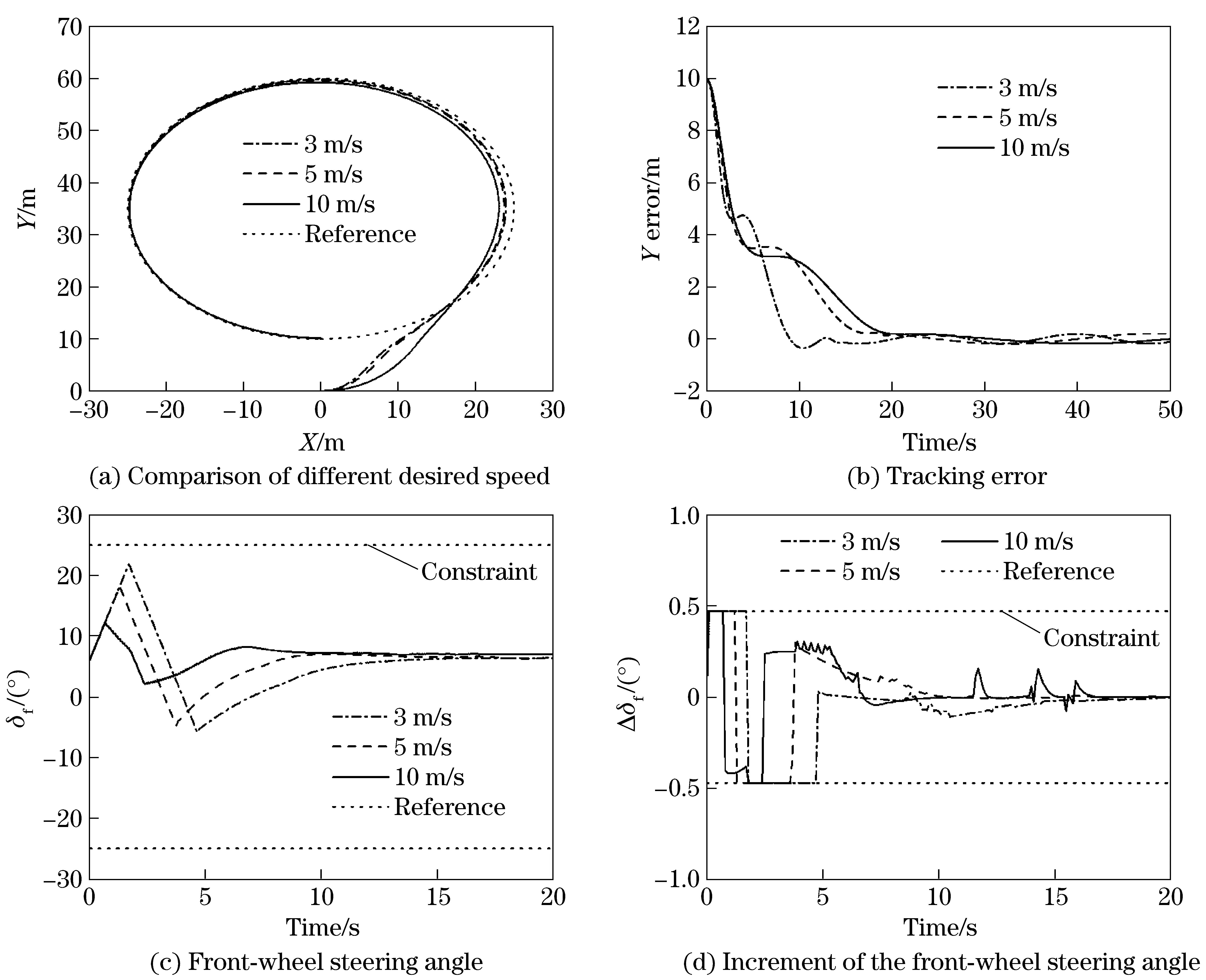
Fig.5 Tracking capability at different desired speed of controller A

4 Conclusions

In this paper,a trajectory tracking controller based on the linear error model MPC is proposed. We apply a softening constraints technique to combine multiple constraints in the MPC objective function. All constraints are generated from the longitudinal and lateral tracking capabilities tests on our real AGV testbed.

The control increment constraint and the relaxing factor in the objective function can ensure the smoothness of control output quantity. The optimal control output sequences of the controller can satisfy the longitudinal and lateral kinematic constraints and actuator constraints. The results of the CarSim/Simulink co-simulation tests show that the controller can track the desired trajectory rapidly and steadily, while satisfying the control limiting constraint and the control increment constraint.

However, as the simplified vehicle kinematic model is taken as the AGV model in this paper and the tire slip and cornering at high speed are not taken into account, the capability of the trajectory tracking controller in the case of high speed is limited. Our future work is to establish a more accurate vehicle model and to test it on our AGV Ray (the champion autonomous vehicle in the China Future Challenge 2013[16]) to further verify the effectiveness of the proposed method, and an initial result of high speed AGV trajectory tracking is illustrated in a video[17].

[1] Jiang Yan, Zhao Xijun, Gong Jianwei, et al. System design of self-driving in simplified urban environments [J]. Journal of Mechanical Engineering, 2012, 48(20): 103-112. (in Chinese)

[2] Wu Weiguo, Chen Huitang, Wang Yuejuan. Global trajectory tracking control of mobile robots [J]. Acta Automatica Sinica, 2001, 27(3): 326-331. (in Chinese)

[3] Jiao Deyu. Robust trajectory tracking control of four-wheel mobile carb [J]. Journal of Jilin University (Engineering and Technology Edition), 2011, (S2):301-305. (in Chinese)

[4] Oriolo G, De Luca A, Vendittelli M. WMR control via dynamic feedback linearization: design, implementation, and experimental validation [J]. IEEE Trans-actions on Control Systems Technology, 2002, 10(6): 835-852.

[5] Cao Zhengcai, Zhao Yingtao, Fu Yili. Trajectory tracking control approach of a car-like mo-bile robot [J]. Acta Electronica Sinica, 2012, 40(4): 632-635. (in Chinese)

[6] Ouadah N, Ourak L, Boudjema F. Car-like mobile robot oriented positioning by fuzzy con-trollers [J]. International Journal of Advanced Robotic Systems, 2008, 5(3): 249-256.

[7] Yang Jun, Ma Rong, Liu Ting, et al. Path tracking of intelligent vehicle based on fuzzy neural network [J]. Computer Simulation, 2012, 29(7): 368-371. (in Chinese)

[8] Cong Yanfeng, An Xiangdong, Chen Hong, et al. Path following control of car-like robot based on rolling windows [J]. Journal of Jilin University (Engineering and Technology Edition)，2012,42(1):182-187. (in Chinese)

[9] Xie Feng. Model Predictive Control of Non-holonomic Mobile Robots [D]. Stillwater, USA: Oklahoma State University, 2007.

[10] Falcone P, Borrelli F, Asgari J, et al. Predictive active steering control for autonomous vehi-cle systems [J]. IEEE Transactions on Control Systems Technology, 2007, 15(3):566-580.

[11] Kuhne F, Lages W F, da Silva Jr J M G. Model predictive control of a mobile robot using linearization [C]∥the 2002 IEEE International Conference on Robotics and Automation, Washington, D C: USA, 2002.

[12] Li Shengbo, Wang Jianqiang, Li Keqiang. Stabilization of linear predictive control systems with softening constraints [J]. Journal of Tsinghua University(Science and Technology)，2010(11):1848-1852.

[13] Jiang Yanhua, Xiong Guangming, Jiang Yan, et al. Design of simulation platform of intelligent vehicular visual odometry based on CarSim and Matlab [J]. Journal of Mechanical Engineering, 2012(22):113-120. (in Chinese)

[14] Li Peng, Wei Minxiang, Hou Xiaoli. Modeling and co-simulation of adaptive cruise control system [J]. Automotive Engineering，2012(7): 622-626. (in Chinese)

[15] Hu Yuwen, Gong Jianwei, Jiang Yan, et al. Hybrid map-based navigation method for un-manned ground vehicle in urban Scenario [J]. Remote Sensing, 2013, 5(8):3662-3680.

[16] Zhu Liwen. The champion autonomous vehicle in the China Future Challenge [EB/OL]. [2013- 05- 01]. http:∥www.bit.edu.cn/xww/mtlg/94665.htm.

[17] Xu Wei. MPC based double shift line trajectory tracking control for a high speed autonomous ground vehicle [EB/OL]. [2013- 09- 03]. http:∥v.youku.com/v_show/id_XNjU3MjQ3ODgw.html.

(Edited by Cai Jianying)

10.15918/j.jbit1004-0579.201524.0403

TP 242 Document code: A Article ID: 1004- 0579(2015)04- 0441- 08

Received 2014- 01- 04

Supported by the National Natural Science Foundation of China (51275041, 61304194); the Doctoral Fund of Ministry of Education of China (20121101120015); the Fundamental Research Funds from Beijing Institute of Technology (20120342011)

E-mail: jiangyan@bit.edu.cn