Ji Zhang(张骥) Kai Liu(刘凯) and Yang Ding(丁阳)

1Beijing Computational Science Research Center,Beijing 100193,China

2Beijing Normal University,Beijing 100875,China

Keywords: microswimmer,confinement,low Reynolds number,creeping flow

1. Introduction

Microswimmers such as bacteria commonly swim in confined spaces such as soils and tissues. The effect of confinement on the mobility behavior of microswimmers has implications in biofilm formation,[1]micro manipulation,[2,3]and biomedical processes,[2,4]hence has attracted continuing research efforts.

Previous studies showed that boundaries and confinement can affect the swimming speed of microswimmers. For example, the forward speed of the sperm decreases monotonically in the pipes until the pipe diameter is small enough to forbid mobility of the sperm.[5]The speed of bimetallic microswimmers can increase up to 5 times due to the electrostatic and electrohydrodynamic boundary effects.[6]Several theoretical and numerical studies have shown enhancement of the swimming speed with confinements in various idealized systems,including dipolar microswimmer,[7]infinite waving sheet,[8]and spherical squirmers.[9,10]

As many microswimmers use helical flagella for propulsion (e.g.,E. coli), the thrust and motion of simple helical structures in confinements have been studied extensively. Including a passive head, Caldaget al.[11]experimentally studied the motion of a magnetically driven helical microswimmer in a pipe. With a fixed geometry of the swimmer, they found that the swimming speed varied little in two cylinders with different radii. Felderhof[12]presented an analytical solution for a slender,infinite helix swimmer in the cylindrical pipe using the perturbation method and reported an enhancement of speed due to the confinement. Liuet al.[13]verified the speed enhancement phenomenon numerically using a boundary element method. They calculated the swimming efficiency of the helical flagella,and found that the optimal geometry is similar to that ofE.coliand does not depend on confinement.

While much is known for the thrust generation and the swimming of simple helical structures driving externally, the influence of the confinement to the speed of self-propelled microswimmers still needs to be clarified.An experimental study by Vizsnyiczaiet al.[14]demonstrated that the forward speed ofE. coliin a square tunnel with a width of about 2.3 µm reaches a maximal speed 1.1 times the free speed. They attributed the speedup to the decrease of the wobbling amplitude due to the confinement. Acemoglu and Yesilyurt studied a self-propelled microswimmer in a finite pipe numerically.[15]The swimmer consists of a spheroid head and a single helical tail. They varied the geometric parameters of the pipe and swimmer and observed a maximum speed enhancement of～30%depending on the ratio of pipe to head radius. However,the assumption that the spin of the tail is a constant relative to the lab frame rather than to the body of the swimmer is unphysical.

Although the speed enhancement of helical swimmers in confinements is repeatedly observed in simulations and experiments, it is still unclear if the enhancement is possible on a self-propelled swimmer purely due to hydrodynamic effects.The dependence of the enhancement in the swimming speed on the geometric parameters of the helical swimmer and the confinement is also not well understood. Here, we develop a numerical model based on a simplified double-helix swimmer in an infinite pipe to study the variation of the speed ratio,and verified the phenomenon experimentally. We further develop a reduced model to extend the ranges of parameters to discuss the optimal geometry that results in maximum speed enhancement,and explore the upper limit of the speed enhancement.

2. Models and validations

2.1. Model system

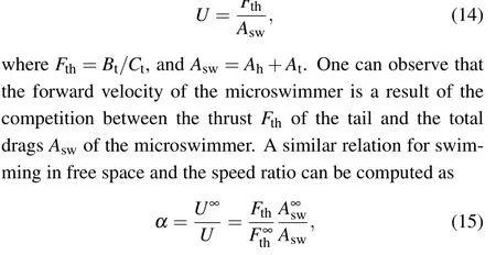
We consider anE.coli-like helical swimmer inside an infinitely long cylinder filled with Newtonian fluid. As shown in Fig.1(a), the microswimmer consists of a rigid cylindrical head with round ends and a rigid double-helical tail.These two parts are connected by a virtual motor that the hydrodynamical effect is negligible. The microswimmer is placed along the pipe center-line. Geometrical parameters of the microswimmer are shown in Fig.1(a),including the radius of the pipeR,the radius of the headrh, the radius of the tailrt, the lengths of the headlhand the taillt=nλ,the pitch of the helical tailλ,the number of periodsn,and the length of the virtual motorδht. We normalize the length of the model using the radius of tailrt.

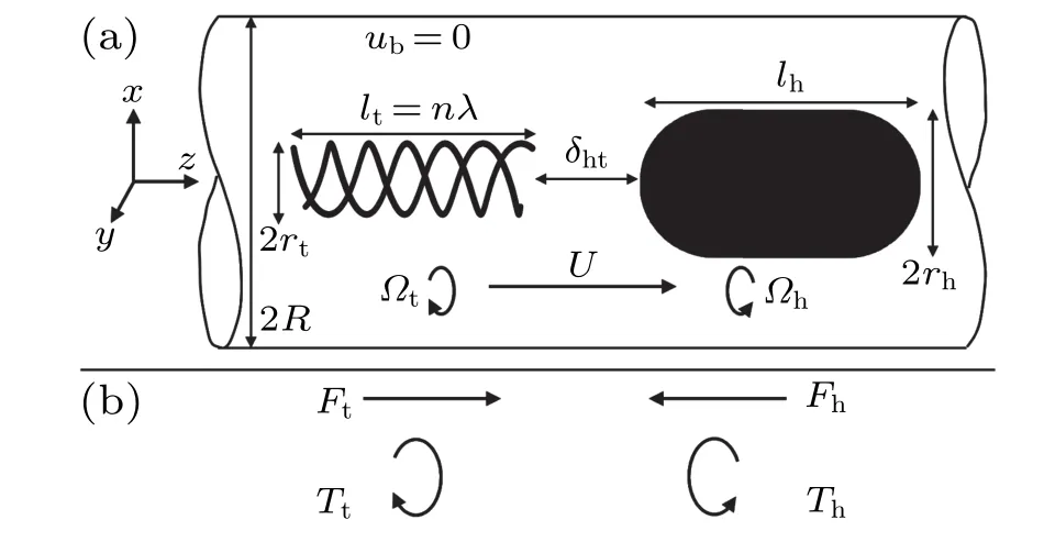
Fig.1. (a)The diagram of the microswimmer in an infinitely long pipe.The microswimmer is placed along the axis of the pipe. The head and the tail rotate in opposite directions. Geometrical and kinetic parameters are illustrated in the figure. (b) Hydrodynamically reduced model of the microswimmer. The forces and torques on the head and tail from the fluid are(Fh,Th )and(Ft,Tt ).

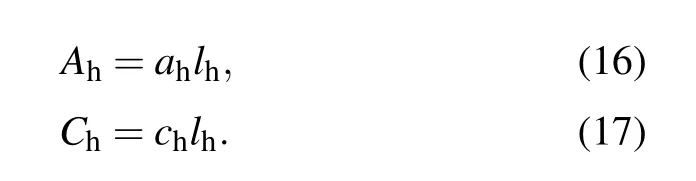
The virtual motor generates a spinΩswthat rotates the head in the counterclockwise direction with an angular speedΩh,and rotates the tail in the opposite direction with an angular speedΩt=Ωh+Ωsw. The rotation of the helix generates a thrust and results in a forward velocityU(R)in the pipe with a radiusR. ThenU∞=U(∞)is the velocity in the free space and the speed ratio is defined as

Due to the symmetry of the body geometry of the swimmer,the translational and rotational velocities of the swimmer have only non-zero components along the axis.

We assume that the fluid moves at the creeping flow regime so that the governing equations of the velocityuare

wherepis the pressure,andµis the fluid viscosity. We apply the no-slip boundary conditions on the surface of the pipe

whererhandrtindicate the relative position of the surface of the microswimmer with respect to the center of the head, respectively. Since inertia is negligible for microswimmers,the self-propelling microswimmer satisfies the force-and torquefree conditions.

The output characteristics of the motor also influence the speed of the swimmer under different confinements,hence influence the speed ratio. Previous studies on several kinds of bacteria have shown that the motors in bacteria have similar output characteristics: at low spin speed the torque is nearly constant and at high spin speed the torque decreases.[16,17]Therefore, we mainly focus on the constant torque case, and without losing generality,we assume unit motor torqueTsw=1. We will also consider the constant-frequencyΩsw=1 and the constant powerPsw=ΩswTsw=1 cases. Taking advantage of the linearity of the system, we only need to scale the speed from one of the cases to get the swimming speeds for the others.

2.2. Numerical solution

We first solve the motion of the swimmer and fluid flow explicitly using the method of Stokeslets.[18,19]We perform full three-dimensional simulations in this study and compute the swimming velocities in all 6 degrees of freedom. We find the lateral component of the swimming speed is less than 0.1%of the forward speed in all cases we tested,consistent with our previous analysis. The linearity of the Stokes equations allows us to decompose the flow fields in terms of fundamental singular solutions of point forces,namely,Stokeslets. By solving a matrix equation connecting the singularity forces and boundary velocities, the flow field and boundary forces can be obtained. Since the relations between the forces and velocities,and torques and angular velocities of the swimmer are also linear, the force-and torque-free equations for the head and tail can be added to the matrix equations for the fluid.[19-21]Then the swimming speed and the rotation of the head and tail can be obtained at the same time as the flow.

The method of Stokeslets has the ability to capture different boundary conditions by applying appropriate Stokeslets.The most commonly used one is the Stokeslets in threedimensional infinite space which connects the velocity at a point in the spacexand a point force atxf.For the Stokeslets in a pipe with zero velocity on the pipe surface,Liron and Shahar have developed a series expression.[22]However, the series expression has a convergence problem when applied to a continuous surface such as the head of the swimmer. To describe the boundary velocity accurately on a continuous surface, the distance of the point force should be small. But the convergence rate of the series is exponentially slow near the point force,especially along the direction of the cylinder axis. We solve this problem by using the series expression for points with large distances from the point force and use free-space Stokeslets(Eq.(7))with corrections from the confinement for nearby points. For the details of reconstructing the Stokeslets in pipe and the validation of the method,see Appendix A.

2.3. Physical model

To verify that a self-propelled swimmer can change speed because of only hydrodynamical effects and validate our numerical models, we developed a physical model - a robot(Fig.2). The shells of the head and the tail are 3D printed using Resin V4 Tough 3D material (Huaxia Plastic Co.). The head radius isrh= 11.2 mm, and the head length islh=123.40 mm. Different from the simulation, a thin rod with radiusρht=2 mm and lengthδht=13 mm is required to connect the motor and the tail. The flagella radius of the tail isρt=2.5 mm.

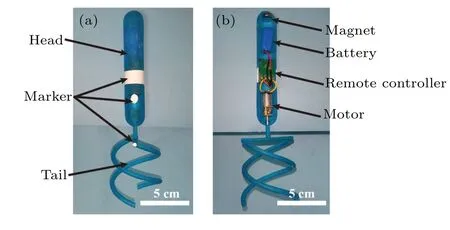
Fig.2. The outside(a)and inside(b)views of the flagellated robot.

We reproduced the phenomena of speedup and slow down by changing the tail shape. Inside the robot head, a motor (model JGA-N20-298, ASLONG MOTOR Co., 40 RPM,11 kg·mm),a remote-controlled infrared switch,and a lithiumion battery (7.4 V, 350 mAH, ZON.CELL Co.) are serially connected (see Fig. 2(b)). A white line and a white dot were drawn on the head of the robot,and a white dot was also drawn on the tail of the robot for video tracking.We adjust the weight of the swimmers by putting in metal chips,such that the robot has neutral buoyancy in the fluid. The neural buoyancy is confirmed by examining the movement of the robot while power off. The speed of the robot in the fluid with the motor off is less than 1%of the speed when the motor is on.

To make the Reynolds number comparable to biological systems, we used silicone oil with a kinematic viscosity of 105cSt. As the robot tail can spin at about 40 rad/min, the corresponding Reynolds number is less than 10-2. We further filled the gaps with silicone grease to prevent the liquid getting into the robot during the experiments. The total depth of the fluid is 500 mm, about four times the robot’s length. We approximate the infinite volume of fluid by using a cylinder with a radius of 147 mm, more than ten times of the robot’s head radius. To minimize the influence of the surface boundary of the fluid, the data was collected when the robot is 150 mm below the surface of the fluid and 150 mm above the bottom of the container. A magnet was used to adjust the orientation of the robot and align its axis with the axis of the cylindrical container before the experiment started. The robot can swim 70-100 mm per minute.The motion of the robot was recorded by a camera at a time interval of 300 ms. We calibrated the image with a scale in the fluid for small optical distortions.The trajectories of the robots were obtained by tracking the markers on the robots. Each case was repeated 3 times.

2.4. Comparison of speeds from experiments and numerical simulations

We compared the speed ratio of two typical kinds of microswimmers,one with a big tail and another one with a small tail. The geometrical parameters of the microswimmers are listed in Table 1.

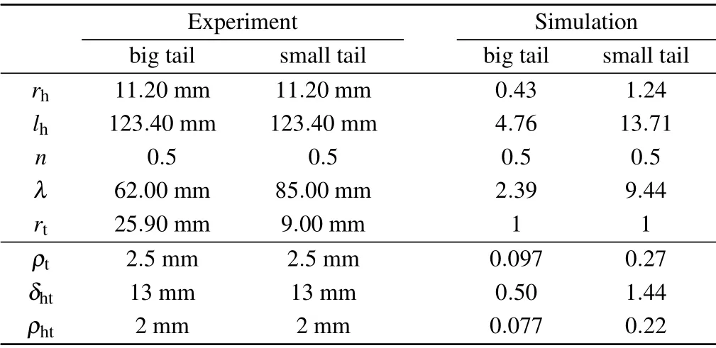
Table 1. Geometric parameters of microswimmers in the simulation and the experiment.

We found that the speed ratio depends on the geometry of the swimmer, especially the ratio of the head size to the tail size. For the swimmer with a small tail, the speed decreases monotonously with the stronger confinement in Fig. 3(a). In contrast,the speed of the swimmer with a big tail increases at first and then decreases as the confinement becomes stronger,as shown in Fig.3(b).

Although there is a system error between experimental and numerical results, the phenomenon is verified, and the speed ratio is close to the simulation results. We attribute the discrepancy to the minor differences in the configurations,such as the connecting rod and surface effects.

The numerical results showed that, for the big tail case,the speed ratio reaches the peak atrt/R ≈1/0.7, consistent with the previous study on a single helix.[13]Since the increase of propulsion is the greatest whenrt/R ≈1/0.7 for the tail,we use this value for the rest of the paper.

Fig.3.The speed ratio α of microswimmer as a function of the ratio between the radius of the tail and the radius of the pipe,defined as rt/R. (a)The microswimmer with a small tail slows down in the pipe. (b)The microswimmer with a big tail speedup in the pipe. The blue dots show the simulation results,and the red dots with the error bar show the experimental results. The labels indicate the pipe radii in the experiments. All the speeds are normalized such that the spin of the motor is a constant 1.

More numerical test cases implied that the length of the tail plays an important role in determining the speed of the swimmer, but the long tails are computationally intensive for numerical simulation. Therefore, to better understand this speedup phenomenon,we developed a reduced model.

2.5. Reduced model

Take advantage of the symmetry, the head and tail can only translate and rotate along the axis of the pipe. Due to the constrain by the connecting rod,Uhead=Utail=U. We further neglect the hydrodynamical coupling between the head and tail and then the motions of the head and tail are related to the forces and torques on them by the following linear equations:[23,24]

The rotation-translation coupling term of the tailBtis an order smaller than other resistance coefficients.[25,26]Ignoring the higher-order termsO(B2t),we have

where the superscript ∞indicates the quantities in the free space.

2.6. Obtain the coefficients of the resistance matrix

A crucial step to calculate the speed ratioαfrom Eq.(15)is determining the resistance coefficients. These coefficients can be obtained from Eqs.(8)and(9)by using the Stokeslets method solving two cases: pure translation{U=1,Ωi=0},and pure rotation{U=0,Ωi=1}for the head and the tail,respectively.

2.6.1. Resistance coefficients of head

The coefficients for the head in the confinement increase linearly with the length when the head is sufficiently long such that the interaction between the head and nearby pipe surface dominates(Fig.4). When the radius of the head is small and short, the confinement effect is weak and a sub-linear (logarithmic)relation is observed. To highlight such transition,we use a relatively small radiusrh/R=0.1 in Fig.4. As the purpose of developing the reduced model is for long head and tail cases, we approximate the forces on the head with linear functions

Quantitatively,our simulation results agree well with the analytical solutions of an infinite cylinder moving inside a pipe:[27]

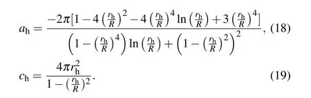
Then the coefficients can be used to extrapolate the resistance of long heads. We note that the effect of the pipe confinement to the rotational coefficient is much weaker than the effect on the translation coefficient(Fig.4(b)).head dragsA∞hin the bulk fluid can not be obtained by taking a limit of Eq.(18). For very large pipe radiusR ≫rh,Eq.(18)gives

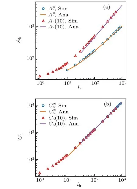
Fig.4. Translational and rotational resistance coefficients of a head in free space(A∞h and C∞h),and inside the pipe with radius rh/R=0.1(Ah andCh).Here rh=1.Solid lines represent the analytical solutions given by Eqs.(16)and(17)(in a pipe),and Eqs.(23)and(21)(in bulk fluid).

For the head in free space,we observed a linear relationship for the rotational coefficient (Fig. 4(b)). Chwang and Wu[28]presented the analytical expression of the torque per unit length of an infinitely long cylinder

In contrast, we observed a sub-linear relationship of the resistance coefficients in the forward direction(Fig.4(a)).The

Alternatively,we can obtain the analytical expression for the head drag based on Ref.[29],in which the drag of a slender body of revolution is provided. Using a constant radius along axis and correcting some typos,the drag on the head is

wherea∞h=2πandβh=ln2-3/2.

While Eqs. (22) and (23) look different, they are actually consistent. There is a competition between the interaction between the pipe and the interaction between different parts of the rod. When the pipe boundary is closer to the head,i.e.,R ≪lh, the confinement effect dominates and the drag increases linearly with length; when the pipe boundary is far from the head, i.e.,R ≫lh, the interaction between different parts of the head dominates and the drag increases sub-linearly with length. The analysis highlights the different trends of head drag with and without confinement,and in the next section, we will show the impact of this difference on the speed ratio.

2.6.2. Resistance coefficients of the tail

From the numerical simulation, we found that the resistance coefficients for short tail increase rapidly, and then the increase becomes slower (Fig. 5). By taking the tail pitchλ=2.5 as an example, we observed a local maximum ofB∞tnearn1≈0.5 (lt≈1.25). Such a maximum is the result of the shadowing of the front part of a helical tail to the posterior part, similar to a previous study.[30]The previous study showed that the speed of the microswimmer with a single helical tail peaks around one periodn1≈1. Since we employed a double-helical tail, the overlap of the projection of the tail perpendicular to the forward direction occurs whenn1=0.5 and causes the local maximum.

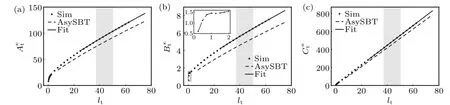
Fig.5. A comparison of the resistance coefficients from the simulation,asymptotic SBT and fitting methods. The translational(a),rotational(b)and coupling(c)resistance coefficients of tail in free space as functions of tail length lt. The inset of panel(b)reports a detailed view of the regions enclosed by the grey dotted box. Tail pitch λ =2.5,tail radius rt =1,and flagella radius ρt =0.1. The gray bars in the background indicate the range where the fittings of cij were done.

To model long tails that require too much computational power and obtain a better understanding of the resistance,we computed the coefficients for infinitely long tails and used these coefficients to approximate the coefficients for long but finite tails. For an infinitely long tail moving along or rotate about its axis, the force is uniform and symmetric about the helix axis. We use the uniform force density to connect the motion of the tail and the total force on the tail. Without loss of generality, we consider a point on one of the helix atx0=(0,rt,0) (see Fig. 6). At this point, the pure translation of the double-helix leads to a local velocityut=(0,0,1)and the pure rotation with an angular speed of 1 corresponds to a local velocityut=(0,rt,0).

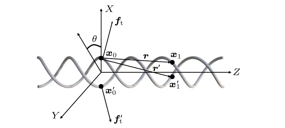
Fig.6. Diagram of the infinite double helix for tail coefficient computation. The angle in XY plane θ ∈(-nπ,+nπ)is used to locate a pair of points(x1(θ)and x′1(θ))on the double helix. Their displacements to x0 are r(θ)and r′(θ),respectively.

The resistance matrixMof the asymptotic theory is a combination of two parts. The first part comes from the contribution of the local forces, andci jare the coefficients. Due to symmetry,the cross-terms related tofrare zero. Further,sincecrris not related to translation along the axis of rotation about the axis,it is not used hereafter. The second part is the long-range contribution of the forces. Since the displacement is dominantly along the axis and the leading term of the coefficient decays as 1/r,only the component along the axis remains,and this term increases logarithmically with the tail length similar to a cylinder. See Appendix A for details of the derivation of the asymptotic analysis.

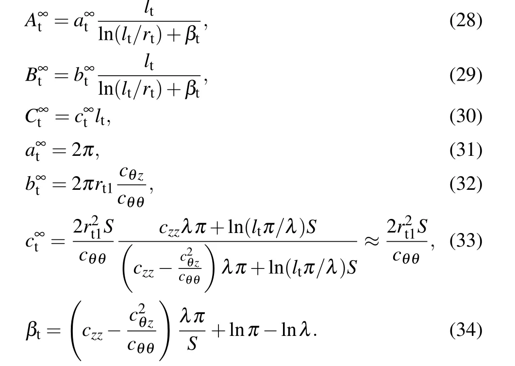
From Eq.(9)and(24)-(27),we obtained the coefficients for a long tail in free space

While the coefficients inMcan be computed using the asymptotic SBT and an overall agreement between the theory and simulation is observed, there are quantitative discrepancies(Fig.5). We attribute the discrepancies to the end effects and approximations in SBT such as the slenderness of the helix. Therefore, instead of using the values from asymptotic SBT, we fit the simulation data using the functional forms of Eqs.(28)-(34). This fitting allows us to approximate the resistance coefficients for longer tails.

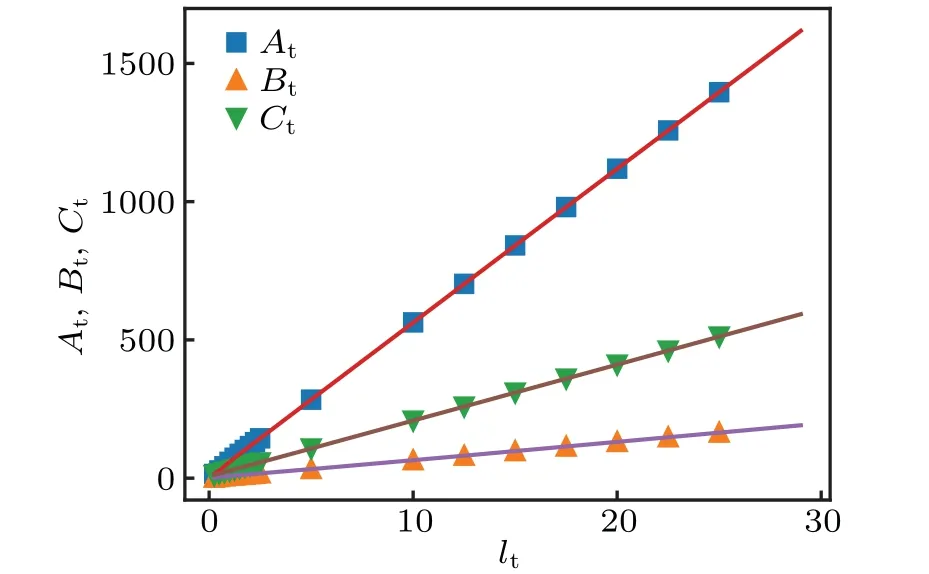
Fig. 7. The resistance coefficients of the tail in a pipe as functions of tail length. R=1/0.7,λ =2.5,and ρt=0.1. The solid lines show the associated linear fitting.

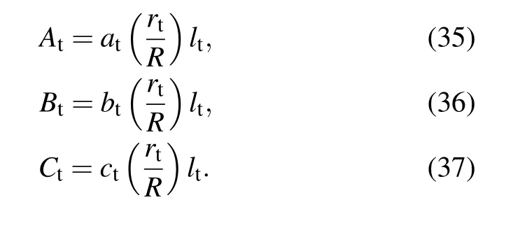
Due to the shielding of the long-range interaction in the pipe, the resistance coefficients for the tail increase linearly with the tail length,i.e.,We fit the simulation results to obtain the coefficients (see Fig.7)and use those values for long tails. Similarly,the accuracy of the linear relationship depends on the length of the tail relative to the radius of the pipe. Since we consider tails that are close to the boundary(rt/R=0.7),the linear relationship is valid for even small lengths.

2.6.3. Error due to the hydrodynamic decoupling

We further tested the reduced model and evaluated the error due to the decoupling using the full numerical simulations. We chose two microswimmers. One has a long head,and the other has a short head. We varied the distance between the head and tail and compared the results from the reduced model with those from the direct simulation(Fig.8).We found that the velocities in general decrease with an increase in the gap length. We attribute the decrease to the shielding effect,[32]which reduces the drag of the microswimmer with a small head-tail gap.For all the cases,the discrepancy between the reduced model and direct simulation is small(<10%),and the velocities converge for a head-tail distanceδhtgreater than about 20. Since the speed ratio measures the relative value between the velocities, the variation inαis amplified, and more significant changes≈20% are observed asδhtvaries.Nonetheless,it converges forδht>20.

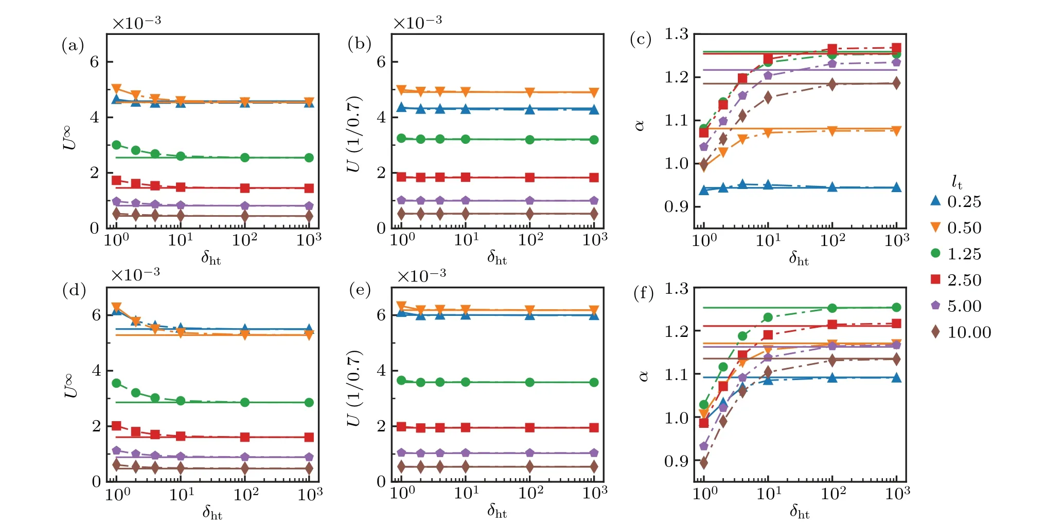
Fig.8. Error due to the decoupling of the head and tail for a long head lh=1.8 swimmer(top row)and a short head lh=0.6 swimmer(bottom row).The velocities in free space U∞(a),(d)and in the pipe U(1/0.7)(b),(e)of the microswimmers,as well as their ratio α(c),(f)as functions of the distance between head and tail δht. The solid lines correspond to the values from the reduced model,the symboles correspond to direct simulations,and the lines are drawn to guide the eye. rh=0.3 λ =2.5,rt=1,ρt=0.1.

In the rest of the study, we combined the numerical method and reduced model to calculate the swimming speeds and speed ratios. Specifically,for short headlh≤80 and short taillt≤25,we employed the numerical method,and for large headlh>80 and taillt>25,we employed the reduced model.

3. Model prediction

To better understand the dependence of the speed ratio on the geometry, we developed analytical approximations of the speed ratioαat the long head and tail limit. First,we summarize the approximations of the resistance coefficients for very long head/tail in Table 2. The resistance coefficients increase linearly in the pipe and logarithmically in free space except for the rotational resistance, which increases linearly with length both inside the pipe and in the free space. Substitute the resistance coefficients in Eq.(15)with those approximations in Table 2,the speed ratio of the microswimmer becomes

Equation(38)indicates that the lengths of the head and the tail appear in pairs and have opposite effects on the ratio.

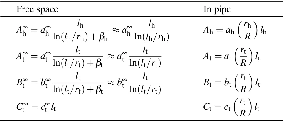
Table 2. The approximations of the resistance coefficients of the microswimmer.

3.1. The optimal geometry for the speed ratio

We first consider the microswimmers with given body slenderness(length/radius). Since many microswimmers have slenderness in the range of 1-100,[33]we used head slenderness of 10 and varied the length of the tail and head.

We observed that moderate head and tail lengths lead to the greatest speedup(Fig.9). Due to the peak of the thrust atn1≈0.5(corresponding tolt≈1.25),the maximum of speed ratio (≈1.3) also occurs near such value for thelh/rh=10 case. For a more slender headlh/rh= 100000 (Fig. 9(b)),the maximal speed ratio is much larger (≈7) and the peak is shifted to longer tail length.

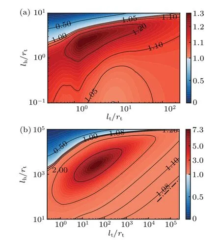
Fig.9. Speed ratio α as a function of the tail length and the head length normalized to the tail radius. Head slenderness, lh/rh =10 in (a) and lh/rh =100000 in(b), is kept a constant in respective subfigures. Tail pitch λ =2.5 and pipe radius R=1/0.7.

We now show that the speedup phenomenon favors a moderate length ratio for both headlhand tailltby considering two extreme cases inside the pipe. At the long head limit,i.e.,lt≪lh, the head dragAhis much larger than the tail dragAtboth inside and outside the pipe,even the head radius might be much smaller than the tail. Then the expression of the speed ratio can be simplified as

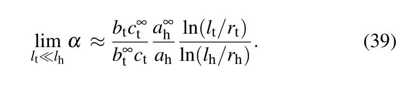
As shown in Eq. (39), the speed ratio increases with increasing tail length. Since the related term ln(lt/rt)comes from the propulsion coefficientB, the physical explanation of this increase is that the increase of propulsion is faster(linear)in the pipe than that in the free space, while the increase of the tail drag is negligible. Correspondingly,the head drag exhibits the opposite behavior.

On the other hand,at the long tail limitlt≫lh,where the drag contributions from the head(i.e.,the terms start witha∞handahin Eq.(38))are negligible. The speed ratio becomes

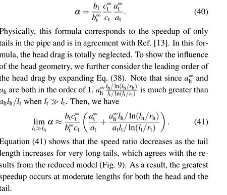
Forlh≫1 andlt≫1, the variations of the logarithmic terms are small and the speed ratio is approximately a constant for the same value oflh/lt. Therefore, the contour line in this regime is approximately straight with a slope of 1(see the right lower corner of Fig.9(b)). The influence of the head radius can also be seen from Eq. (41). When the tail is very long, and the head radius is small, the increase of the head radius leads to a perturbation that increases the speed ratio.When the head radius is large enough, the gap between the head and the pipe is tinny. The lubrication theory predicts that the drag force diverges.[27]Therefore,the speed ratio is maximized with a small but finite head radius.

3.2. Upper limit of the speed ratio

Obviously,the lower bound of the speed ratio is zero. For example, a microswimmer with a thick head can move in the free space but will get stuck in the pipe. In this subsection,we vary the slenderness of the head and discuss the maximal value of the speed ratio.We will show that the speed ratio has no upper bound by constructing certain geometries of the swimmer and associated analytical expression of the speed ratio. The key is to make the head drag much larger than the tail drag in the bulk fluid and keep the head drag comparable with the tail drag in the pipe.

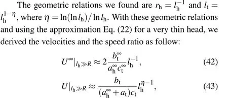
Fig.10. (a)The speed ratio as a function of head length lh when the head radius varies as rh=l-1h and tail length varies as lt=l1-ηh . (b)The velocities inside the pipe and in free space as functions of the speed ratio.

3.3. Influence of the motor output characteristics

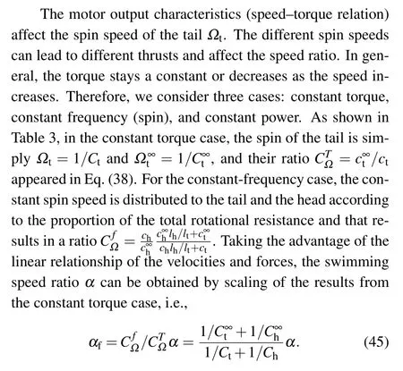
Since the resistance coefficients in the pipe are always greater than those in free space,it is easy to see thatαf>α.

As show in Fig. 11, the overall profile is similar to the constant torque case (Fig. 9). As the power is the product of spin speed and torque,the case of constant power can be considered as an average of the constant-frequency and constant torque cases. Therefore, for some swimmers, at least including those withα>1 in Fig.9,the cost of transport in terms of energy consumption per distance is lower in the pipe than that in the free space.

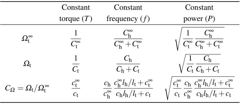
Table 3. Influence of motor output characteristics on the spin speeds ofthe tail and their ratio.

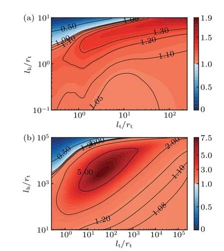
Fig. 11. Speed ratio as a function of the tail length and head length.Motor spin speed Ωsw is a constant 1. Head slenderness,lh/rh=10 in(a)and lh/rh=100000 in(b),is kept a constant in respective subfigures.Tail pitch λ =2.5 and pipe radius R=1/0.7.

4. Conclusion

In this study,we investigated the speedup of microswimmers in a confined environment-an infinitely long pipe. Using numerical simulation and robotic experiments,we showed that a free swimmer can speedup in such confinement purely due to hydrodynamic effects. By developing a reduced model and analyzing the propulsion and drag forces on the head and tail, we showed that the speed ratio is maximized by a moderately long head and tail. While the speedup for a swimmer with realistic geometry is small, theoretically, the speed ratio has no upper limit when the lengths of the head and tail increase with a certain proportion and head slenderness. Our results highlight the shielding effect on the interactions between different parts of the swimmer. Such a mechanism might also influence the locomotion in other confined environments. We also showed that the virtual motor that generates a constant frequency could lead to a greater speedup compared with a virtual motor that can generate a constant torque.

The bacterial tails are usually flexible. The helical shape is formed due to the coupling between the driving torque and force from the motor, internal elastic forces, and drag forces from surrounding fluids.[34-36]Our study is limited to a fixed shape to focus on the hydrodynamic effect due to the confinement. How confinements affect the shape and locomotion performance of realistic flexible tails will be studied in the future.

Acknowledgments

Project supported by the National Natural Science Foundation of China (Grant Nos. 11672029 and U1930402). We thank Xinliang Xu, Ebru Demir, and Martin Stynes for helpful discussions and carefully reading the manuscript. We acknowledge the computational support from the Beijing Computational Science Research Center.

Appendix A:The Stokeslets method in a pipe

First, here we recapitulate the Stokeslets method. Consider a Stokes flow with a point forceflocated atxfin the regionΩ. The governing equation of the velocityureads as

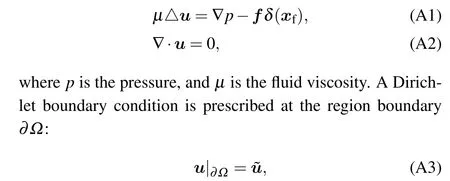
where ˜uis a given velocity.

The principle of the Stokeslets method is to place many known solutions of point forces on the boundary or somewhere outsideΩ,called StokesletsSkn,then find the strength of these Stokeslets that generate the desired boundary velocity. One of the most commonly used Stokeslets is the one in three-dimensional infinite space:

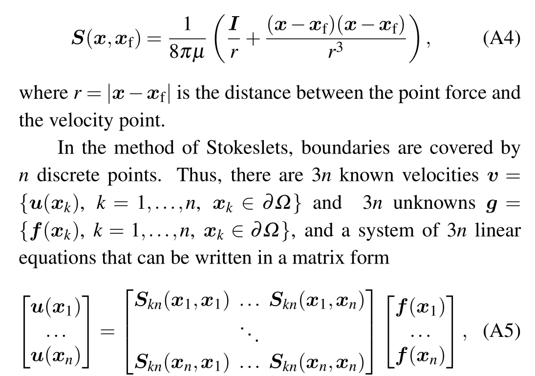
or

The matrix equations were solved using the generalized minimal residual method(GMRES)in this study.Once the strengthgon the boundary is obtained,the velocity at an arbitrary locationxcan be calculated by

Series solution of the Stokeslets in a pipe

Here we develop the Stokeslets in a pipe based on the series solution of a point force given by Liron and Shahar.[22]The velocities at the pipe boundary and infinity are zero:

In cylindrical coordinates, the expression of the velocity atxu=(r,φ,z) due to a point force located atxf=(b,0,0) in the pipe(see Fig.A1)is

whereupipe=(uR,uφ,uz)is the velocity vector,Pk,nandQk,nare complex functions of the modified Bessel functions of the first kindIk(s) and the second kindKk(s), respectively. The details can be find in Appendix B of Ref. [22]. In Eq. (A9),bn,k=Im(xn,k), andcn,k=Im(yn,k), where Im(•) means the imaginary part of•.xn,kandyn,kare the complex and imaginary roots of Eq.(A6)in Ref.[22]:

SinceIk(s)=I-k(s)whenk ∈Z,xn,-k=xn,kandyn,-k=yn,k.In this study,the roots of Eq.(A10)in the rangesk=0-1000 andn=1-1000 were solved and stored.

Fig. A1. Schematics of the Stokeslets in a pipe. A cylindrical coordinate(r,φ,z)is employed in the system.The a dotted line represents the axis of the pipe,which coincides with the z. The point force is located at xf=(b,0,0).The pipe is cut into three parts by two imaginary surfaces A1 and A2 (indicated by dash-dotted lines) and are labeled as Ω1, Ω2 and Ω3. The regions Ω2,and Ω3 are semi-infinite and the length of Ω1 is L.

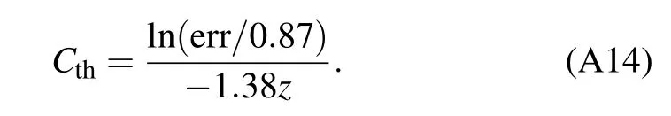
Next, we examine the convergence of the series solution and show that the converges for smallzare too slow to be used directly. There are two exponential decays in the series solution, and the associated coefficients arebn,kzandcn,kz. As shown in Fig.A2,both these two coefficients increase monotonically withnandk,but the increase withkis approximately two times faster than that withn. Therefore,we choose cutoff thresholds differently forkandnsuch that values of the last componentsbn,kandcn,kare approximately the same to avoid the useless computation. As shown in Figs.A2(c)and A2(d),with the same cutoff valueCth,the values forbn,kandcn,kare about the same. Then the infinite series become

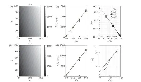
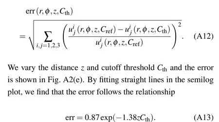
Fig.A2. Convergence test of the Stokeslets in a pipe. (a)and(b) The contour plots of bn,k and cn,k as functions of n and k, respectively. (c)and (d) The values of bn,k and cn,k as functions of the cutoff value Cth,respectively. (e)The error of the velocity at different positions and cutoff parameters. The solid line,with a slope of-1.3648,is the best linear fit of the data. (f)The time required for computing the series expression. The solid line is the best linear fit of the data,and its slope is 1.87.

A point forcef= (0,0,1) located atxf= (0.5R,0,0)is selected in the test. We chose the velocity value fromCref=1000 as the reference solution and the relative error for cutoffCthis computed as

Therefore,for given err andz,the requiredCthis

The computational cost includes two parts: obtaining the roots of Eq. (A10), and the summation in Eq. (A11). Since the roots can be solved just once and stored, the only timeconsuming part of the computation is the summation. The average time to compute 1000 times ofSpipeon a computer with Intel(R) Xeon(R) CPU E5-2680 v3 @ 2.50 GHz is shown in Fig.A2(f). We observed that the time increases near quadratically withCth. If we set a goal for the maximal error as err=10-3,the computational time required forz=0.01Randz=0.001Ris 98 seconds and more than two hours, respectively. As we need to cover the surface of the whole body with the Stokeslets,such time consumption is unacceptable.

Reconstruct the Stokeslets in pipe

In this section,an analytical-numerical combined method is used to solve the smallzproblem raised above. As shown in Fig.A1,the pipe is cut into three regions by two planesA1 andA2. The middle region contains the point force. The series expression converges rapidly in the other two regions and does not require special treatment. The goal is to obtain the StokesletsSpipenumerically in the middle regionΩ1.

As a tensor,Spipecan be obtained by the calculation of three orthogonal velocity components for point forces along the three axes. The boundary condition ˜uconsists of three parts,i.e.,ub=0 on the pipe wall,uA1on the imaginary wallA1,anduA2on the imaginary wallA2. Since we can compute the velocity onA1andA2accurately using the series expression,their values are known.

To remove the singularity inΩ1and make the Stokes equation satisfied everywhere, we subtract the velocity field from a point force in free space and add it back later. The residual velocityuires(x,xf)is

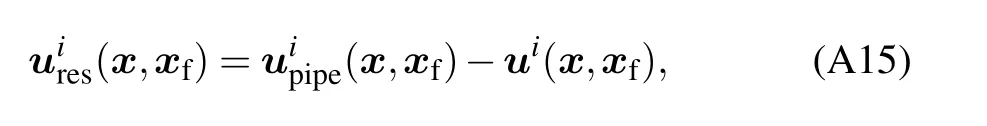
whereui(x,xf)=Sfis the singular velocity field due to a unit point forceei(xf) in free space (see Fig. A3(b)), The residual velocity field cancels the velocity at the pipe surface.The problem is reduced to finding the residual velocity field numerically that satisfies the boundary condition ˜uires(xf)(see Fig. A3(c)). The force distributiongreson the boundary for this residual velocity field can be solved with the Stokeslets method.

Fig.A3. Schematics of the numerical method for reconstructing the Stokeslets in Ω1. (a)The Stokes problem in a finite pipe with a singular unit point force f located at xf and given boundary condition ˜upipe. The fluid field (Stokeslets) induced by f can be decomposed into a singular part(b)and a harmonic part(c). (b)The flow induced by the Stokeslets in free space S. The velocity on the imaginary boundary is ˜u.(c)The Stokes problem with the boundary condition ˜ures= ˜upipe- ˜u.

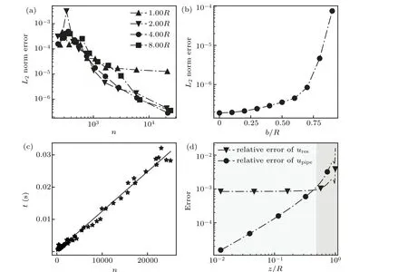
Fig.A4.The convergence test of the reconstructed Stokeslet.(a)The L2-norm errors of the boundary velocity as functions with the total of the Stokeslets n on the boundary of the finite pipe Ω1 with different lengths. In this test case,a unit point force f =(0,0,1)is located at xf =(0.5R,0,0). (b)The L2-norm error of the boundary velocity as a function of the location xf=(b,0,0)of a unit point force f =(0,0,1). (c)The computational time of using the Stokeslets in pipe as a function of the total number of Stokeslets used on the boundary in the reconstruction process. (d) A comparison between the velocities on the line(0.5R,0,z)computed using the series expression uaz na and using the reconstruction method unz um. The relative error of ures,z is computed as||(uarensa, z-unreusm,z)/uarensa,z||. The relative error of upipe,z is computed as||(uapnipae,z-unpuipme,z)/uapnipae,z||.

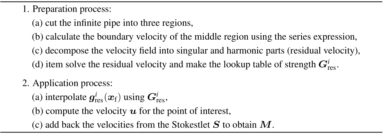
Table A1. Steps of reconstructing and using the Stokeslets in a pipe.

A technical problem is to find proper pipe lengthL. We examined the accuracy of the numerical method for different pipe lengths and the number of force points on the boundary. We placed 6000 random points on the boundary of the finite pipeΩ1, and calculated theL2-norm error. As shown in Fig. A4(a), theL2-norm error of the short pipe (L=R) is significantly worse than other cases. This is because of the complex velocity profile on the surfacesA1andA2.Therefore,we choseL=2Rin this study.

The strengthgresfor the residual field is a function of radial location of the point force. We found that the error increases significantly whenb>0.8 and becomes computational demanding (Fig. A4(b)). To speedup the numerical method, we made a lookup table forgres. Particularly, we computedgires(xfl) for a point atxfl, wherexfl=(bl,0,0).bl= 0,...,0.8, wherel= 0,1,...,800. The lookup table contains all solved values of the point forces is denoted asGires={gires(xfl)}. Then a spline interpolation was employed to calculate the strengthgires(xf) from the stored lookup tableGires. The StokesletsSpipecan be reconstructed once the residual velocity fieldsuiresare computed by adding back the Stokeslet in free space. A summation of the reconstruction process is listed in Table A1.

The computational time increases linearly with the number of Stokeslets in the reconstruction process(see Fig.A4(c)).In this study,we placed 9214 point forces on the boundary of the finite pipeΩ1.

To test the accuracy of the reconstructed velocity field,we placed the point force(0,0,1)at(0.5R,0,0)and calculated the relative error ofuresandupipe(Fig. A4(d)). The relative errors ofuresare small in the range||z||<0.5(light gray area in Fig.A4(d))but increase for largezdue to the discretization on the boundary. Contrary to the series expression,the reconstructed Stokeslets in pipe have higher accuracy near the point force. Therefore, the series expression of the Stokeslets was used for||z||>0.5.

Resistance coefficients of an infintely long tail in free space

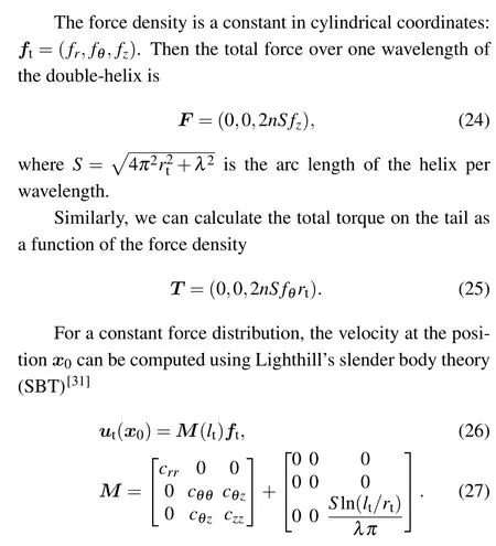
As shown in Fig.6,we considered a double-helix moving in free space and computed the resistance coefficients for axial translation and rotation. Now we calculate the force densityftusing Lighthill’s slender body theory.[31]Without loss of generality, we set the viscosity of fluidµ ≡1 in this study. We assume that the length of the double-helixltis long enough such that the force density is a constant in cylindrical coordinates,i.e.,ft=(fr,fθ,fz),and the end effects are negligible.The force on one of the helices in Cartesian coordinates can be obtained by coordinates transformation Here,Sln(lt/rt)/(λπ) represents the nonlocal effects along the axial direction.

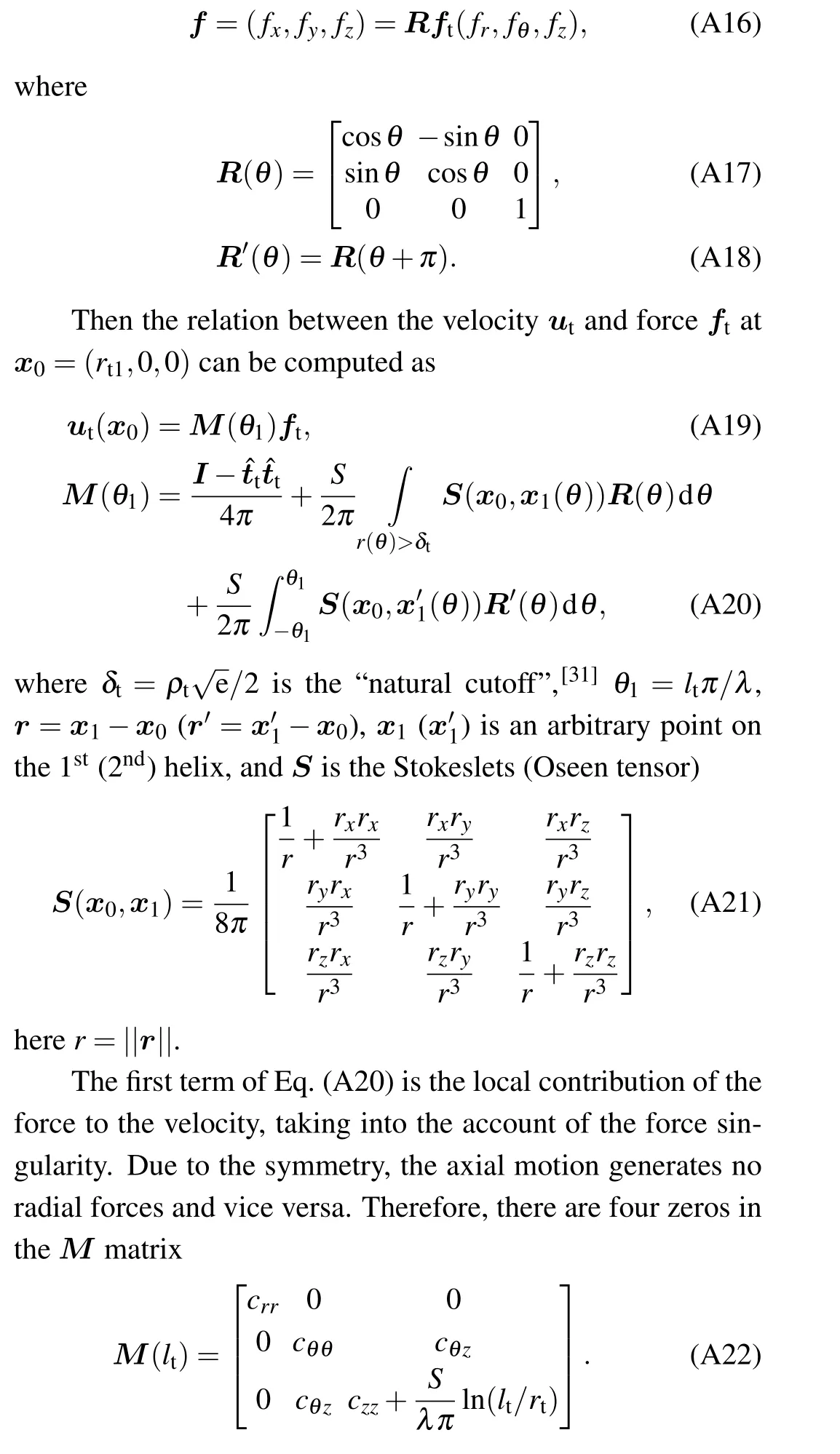
The local contributionci jof theMmatrix can be integrated numerically.For instance, withrt= 1,ρ= 0.1, andλ= 2.5, we obtained (crr,cθθ,cθz,czz) =(0.09416,0.51779,0.03036,1.16631).