Sha Lou (娄厦), Shu-guang Liu , (刘曙光), Gangfeng Ma , Gui-hui Zhong (钟桂辉), Bo Li (李博)

1. Department of Hydraulic Engineering, Tongji University, Shanghai 200092, China

2. Key Laboratory of Yangtze River Water Environment, Ministry of Education, Tongji University, Shanghai 200092, China

3. Department of Civil and Environmental Engineering, Old Dominion University, Norfolk, VA, USA

4. School of Engineering, Nagasaki University, Nagasaki, Japan

Introduction

The complex interactions between the surface water and the groundwater are found in coastal areas.The infiltration and the exfiltration on the beach faces may influence the contaminant exchange between these two systems and the sediment transport on the beaches. On the other hand, the nearshore hydrodynamics affected by tides and wave setups play an important role in the subsurface beach flow and the groundwater table fluctuation in coastal aquifers[1].

Although the surface water and the groundwater are hydraulically interconnected, they are usually considered as two independent systems and analyzed separately. The simple approach to account for the influence of tides on the groundwater flow is to run the groundwater model using a boundary condition at the beach face with a temporally varying hydraulic head. For instance, Pauw et al.[2]implemented this approach with the SEAWAT model to study the impact of tides on the groundwater flow in unconfined coastal aquifers. Lee et al.[3]implemented a similar approach with the FEEFLOW model to investigate the relationship between the periodic sea level change and the submarine groundwater discharge rate in a coastal aquifer. Post[4]applied a periodic boundary condition with the MODFLOW to simulate coastal groundwater systems. Li et al.[5]also developed a numerical model to study the beach groundwater table fluctuation based on the tidal dynamics. In all these studies, the governing equations of the groundwater flow were solved using a free and moving boundary condition on the beach face accounting for the seepage dynamics as well as the tidal level variations.

To simulate the effects of the wave dynamics on the groundwater flow, a surface water model for the nearshore wave propagation and transformation is needed. The one-way coupling between the surface water model and the groundwater flow model is adopted by most researchers. For example, Bakhtyar et al.[6]coupled a variable density groundwater flow model with a nearshore hydrodynamic model, where the nearshore hydrodynamic model was used to capture the wave motion, and to provide the hydraulic head on the beach boundary for the groundwater flow modeling. Geng et al.[7]developed the MARUN model to simulate the density-dependent groundwater flow under the impacts of waves, where the wave propagation in the nearshore was simulated by a CFD solver FLUENT. Their study revealed that the waves might generate seawater-groundwater circulations in the swash and surf zones. Li et al.[8]proposed a process-based numerical model BeachWin, which is capable of simulating the interactions between the waves and the subsurface beach flow, where the depth-averaged nonlinear shallow water equations were solved for the wave motion. In all above-mentioned models, one-way coupling strategy is adopted to account for the interactions between the surface water and the groundwater. The groundwater flow is driven by a temporally-varying hydraulic head on the beach face, which is computed by a surface water flow model. The groundwater flow has no feedback on the nearshore hydrodynamics.

In order to better simulate the interactions between the surface water and the groundwater, an integrated surface water and groundwater modeling approach was proposed recently. Yang et al.[9]used the HydroGeoSphere model to simulate the effects of the tides and the storm surges on the coastal aquifers,where the coastal flow was simulated with the diffusive-wave approximation of the St. Venant equation on the two-dimensional surface. Richards’ equation and Darcy’s law were used to solve the three-dimensional saturated, variable-density groundwater flow. In the HydroGeoSphere model, the subsurface domain was represented by horizontally oriented three-dimensional prismatic finite elements of unit thickness,while the surface domain was described by twodimensional rectangular elements. It was assumed that there was a thin layer on the interface between the groundwater and the surface water, and a dual node approach was used to calculate the water exchange across the interface. Although the surface water and the groundwater were fully coupled, the governing equations and the discretization schemes were still separated in the surface water and groundwater domains. Liang et al.[10]established a dynamic linkage between the vertically averaged surface water and the groundwater flows. The sub-models for the free surface and subsurface flows were combined horizontally. The governing equations for the surface and subsurface flows were solved simultaneously within the same numerical framework, and both the mass and momentum transfers were considered. However, the two dimensional shallow water equations were obtained through the integration over the depth and adopted for the surface water flow neglecting the viscous forces. For the groundwater, the two-dimensional Boussinesq equations were used according to the Dupuit-Forchheimer assumption[11]. Its application was restricted to the flows in an isotropic, homogeneous, and unconfined aquifer. Yuan et al.[12]developed an integrated surface and groundwater model with a moving boundary on a fixed numerical grid. A hydrostatic pressure distribution in the vertical direction is assumed and the three-dimensional Reynolds-averaged equations are integrated over the depth of the water, resulting in simplified two-dimensional equations. An explicit method and a semiimplicit scheme were then used to solve the governing surface and subsurface flow equations, respectively.Based on this work, Kong et al.[13]developed a numerical model for the integrated surface water and groundwater. The surface water domain and the groundwater domain were combined horizontally. The surface water and groundwater flows were coupled through the source/sink term to account for the discharge across the interface under the hydrostatic pressure assumption. The convection terms of the momentum equations were considered for the surface water. On the beach face where the surface water and the groundwater coexist, the groundwater depth was determined by the local aquifer depth. Similar methods were also employed by Yuan and Lin[14],Bakhtyar et al.[15]. In these models, the equations for the surface water and the groundwater were assembled into one single set of linear algebraic equations and were simultaneously solved. The pressure distribution,which is a sensitive issue for the wave motion in coastal areas, was however assumed to be hydrostatic over the whole water depth.

Therefore, the development of a fully integrated three-dimensional non-hydrostatic surface water and groundwater model is desirable to further analyze the interactions between the surface water and the groundwater flows in coastal areas. This paper proposes an improved fully integrated model based on the nonhydrostatic wave model NHWAVE[16]to simulate the tide and wave processes in the permeable sandy beach.The NHWAVE was well validated for the nearshore wave dynamics, and was applied to study the wavevegetation interactions[17], the tsunami waves generated by the submarine landslides[18], the rip currents in the field-scale surf zone[19], the wave interactions with the porous structures[20]as well as the infragravity wave dynamics in fringing reefs[21]. In this paper, the NHWAVE model is applied to solve the well-balanced Volume-averaged Reynolds-averaged Navier-Stokes (VARANS) equations. The spatially varying porosity and hydraulic conductivity are introduced to identify the domains for the surface water and the groundwater. The model is utilized to obtain results to compare with the laboratory measurements reported in the literature, involving the tide propagation through a sandy embankment, the tide-induced groundwater table fluctuation in a sandy beach, and the wave setup in a sloping sandy beach. The dynamic interactions between the surface water and the groundwater are discussed, and the influences of the tides and the waves on the groundwater flow are analyzed.

1. Model equations

The implementation of the fully integrated surface water and groundwater flow model in the NHWAVE is based on the VARANS equations[22],obtained by using the macroscopic approach for a mean behavior of the flow field in the porous media by averaging its properties over the control volumes.The formulations of the VARANS are given by del Jesus et al.[22]as

where (i,j) =(1,2,3),xi*is the Cartesian coordinate,uiis the velocity component in thex*jdirection,nis the porosity,p0is the total pressure,ρ is the water density,gis the gravitational body

iforce, and ν and νtare the laminar and turbulent kinematic viscosities, respectively.

The forcing termRui/nin Eq. (2) comprises three parts in the porous structures with a large porosity[22]: the frictional forces, the pressure forces,and the added mass. In the sandy beach, where the porosity is relatively small, the pressure forces and the added mass are negligible. Thus, only the frictional forces are considered in this paper.Ris related to the hydraulic conductivity.

Clearly, the above equations are valid for both surface water and groundwater flows. If the porositynis equal to unity, Eq. (2) is degraded to the traditional Navier-Stokes equations. In a porous media with a low porosity, the flow velocity is usually small,and therefore the advection and diffusion terms in the momentum equations are negligible. Eq. (2) can then be reduced to the famous Darcy’s law.

where= -p+ ρgi(with indices not summed) is the effective pressure,K=g/Ris the hydraulic conductivity, andqi=ui/nis the Darcy flux.

In the NHWAVE, the governing equations are solved in a σ-coordinate system. With the coordinate transformation, Eqs. (1), (2) can be written in a conservative form as

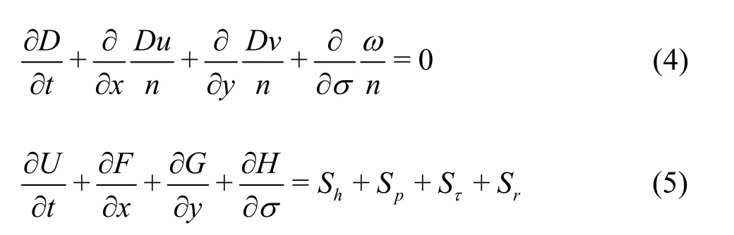
where

The fluxes are

The source terms are given by

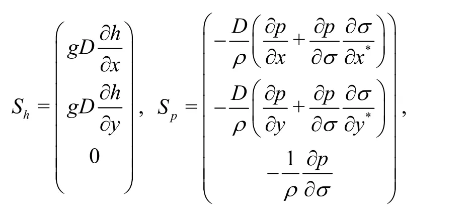
where the total pressure is divided into two parts: the dynamic pressurep(withpas the dynamic pressure for simplicity) and the hydrostatic pressure ρg( η -z).Dis the total water depth (water depthhplus surface elevation η), and (u,v,ω) are thex,y,σ components of the velocity.

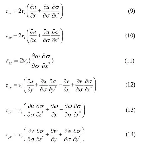
The turbulent diffusion termsSτx,Sτy,Sτzare given by

The stresses in the transformed space are calculated as

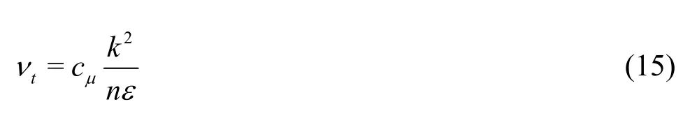
The turbulent kinematic viscositytν is calculated by the -kε turbulence closure. The volumeaveraging approach can also be applied to the -kε equations. The Darcy’s volume-averaged eddy viscosity is calculated as

The -kε equations in the conservative form are given by

wherekand ε are the Darcyʼs volume-averaged turbulent kinetic energy and the turbulent dissipation rate, respectively.k∞and ε∞are the closures for the porous media flow, which are negligible in the case of low porosity. σk=1.0, σε=1.3,C1ε=1.44,C2ε= 1.92 andCμ= 0.09 are empirical coefficients[23].PSis the shear production, which is computed as

where the Reynolds stressis calculated by a nonlinear model for the porous media flow, which is further modified to include the porosity inside the derivatives, yielding the following form.

in which the flow velocity=u/n, andC,C,id1C2andC3are empirical coefficients[20].

2. Results and discussions

2.1 Tide propagation through a sandy embankment

The fully integrated NHWAVE model is employed to obtain results to compare with the laboratory measurements of Ebrahimi[24], in an idealized experiment to study the tide propagation through a sandy embankment. Figure 1 shows the study domain and the longitudinal section of the tidal lagoon experiment.The velocity variations on Section A and the water elevations on both sides of the embankment (Section B and Section C) were monitored in the laboratory experiment. To study the linkage of the separated surface waters on the two sides of the embankment, a sinusoidal tide is specified on the left boundary of the domain. The tidal amplitude and period are 0.006 m and 355 s, respectively. The hydraulic conductivity and porosity of the non-cohesive sand in the embankment are 0.0001 m/s and 0.3, respectively. All parameters take the same values as those in the laboratory experiment. The model is established with a grid size of 0.020 m, and ten vertical sigma layers in the vertical direction. The initial water depth is 0.027 m to indicate a high water level scenario. The time step is determined at every time step based on the Courant-Friedrichs-Lewy (CFL) condition.

To simulate the influence of the tidal flow on the water body inside the lagoon by the groundwater seepage, the velocity at Section A and the water elevations at Section B and Section C are examined.The comparison of the measured and simulated velocities at the middle point of Section A is shown in Fig. 2 (uis the velocity,tis the time). The agreement between the measurements and the simulations is excellent with only a slight difference at the low water level. The relative errors are about 7.7%-14.3%at the tidal wave troughs. The simulations agree with the measurements much better at the wave crests.Figure 3 shows the changes of the water elevation relative to the mean water depth on both sides of the embankment (Sections B and C). The measured and simulated water elevations agree perfectly with each other on both sections. At the first two cycles, both the measured and calculated elevations decrease dramatically behind the sand embankment with a very small discrepancy. The phase lag between the water surface oscillation in the lagoon and the tidal oscillation in the coastal region is about 90°.

Figure 4 shows the longitudinal variations of the surface water elevation on both sides of the embankment and the groundwater table inside the embankment at typical moments within one tidal cycle.Line a in Fig. 4 stands for the surface water elevation and the groundwater table at a high water, and lines b-c-d are those at the moments followed with a 1/4 cycle interval. The oscillation of the water level in the lagoon responding to the periodic tide can be observed.

Fig. 1 Longitudinal section of study domain in the tidal lagoon experiment (m)

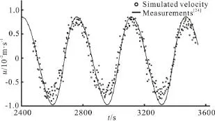
Fig. 2 Comparison of measured and simulated velocities at the middle point of Section A

Fig. 4 Simulated longitudinal variations of surface water elevation and groundwater table at typical moments during one tidal cycle

As shown in lines a and b, when the surface water elevation starts to decrease from a high level during the ebb tide in the coastal region, the water level in the lagoon keeps increasing. At a static water, the surface water elevation in the lagoon reaches the highest. The groundwater table inside the embankment also sees significant changes during this process. The groundwater table on the coastal side becomes lower, while it becomes higher on the lagoon side. The intersection is located at about 3/4 length along the groundwater table from the coastal side. From line b to line c, when the surface water elevation continues to decrease in the coastal region, the water level in the lagoon turns to fall, and this trend continues in the remaining tidal cycle till the water level in the coastal region reaches the static water again. The difference between the surface water levels in the coastal area and the lagoon side is the smallest at the static water shown in line d,and the groundwater table is relatively lower in the middle of the embankment at this moment. The results in Fig. 4 demonstrate the effect of the groundwater on the surface water. The slow groundwater flow inside the embankment results in the phase lag between the surface water elevations on two sides of the embankment. The variation of the surface water level also has an influence on the groundwater table. The change of the groundwater table on the coastal side is more significant than that on the lagoon side.

Fig. 5 Longitudinal variations of surface water elevation and groundwater table with different values of hydraulic conductivity

To further analyze the variations of the surface water elevation and the groundwater table affected by the embankment, two test simulations for different values of hydraulic conductivity are conducted. In Test 1, the hydraulic conductivity is 0.001 m/s, which is ten times smaller than that in the laboratory measurements. Test 2 has a larger hydraulic conductivity of 0.005 m/s. Results of the longitudinal water elevation variation at typical moments during one tidal cycle in two tests are shown in Fig. 5 (his the water elevation). In Fig. 5(a), the amplitude of the groundwater table inside the embankment decreases significantly from the coastal side to the lagoon side. The surface water elevation in the lagoon is barely affected by the tides in the coastal region. The small hydraulic conductivity makes the embankment act like a barrier to prohibit the groundwater flow from affecting the lagoon. In Fig. 5(b), with a larger hydraulic conductivity, the amplitudes of the groundwater table inside the embankment and the surface water elevation in the lagoon side are close to each other, both of which are slightly smaller than the tidal amplitude in the coastal area. With a large hydraulic conductivity, the groundwater flows sufficiently fast to keep the groundwater table inside the embankment and the surface water in the lagoon at the same phase as that of the tide in the coastal area.

Fig. 6 Simplified layout of the experiment investigating the tide-induced groundwater table fluctuation under a rectangle beach and the locations of measurement sections(m)

Although the values of the hydraulic conductivity in Test 1 and Test 2 can hardly compared with the real material feature of the embankment, the results in Figs.4, 5 indicate that the hydraulic conductivity is a significant parameter for the groundwater dynamics.The groundwater table is extremely sensitive to the hydraulic conductivity. With a larger hydraulic conductivity, the phases of the groundwater and the surface water are closer to each other and the surface water on the lagoon side is more active.

2.2 Tide-induced groundwater table fluctuations inside a rectangle beach

A laboratory experiment to analyze the groundwater table in a porous medium driven by an oscillating water level[14]. In this experiment, a simplification is made for the groundwater table fluctuations to be considered inside a rectangle beach due to the tidal motion as shown in Fig. 6. The experimental data are used to verify the simulated results obtained by using the modified NHWAVE model in the present study. In the numerical model,the water level oscillates in a sinusoidal manner on the left boundary as the tidal motion. The remaining boundaries are assumed to be solid vertical walls. The mean water depth is 0.028 m. The tidal period is 35 s and its amplitude is 0.090 m. The hydraulic conductivity and the porosity of the sand in the beach are 0.0001 m/s and 0.345, respectively. The grid size is 0.010 m, and ten layers are employed in the vertical sigma-coordinate. The time step is determined in every calculation interval according to the CFL condition.

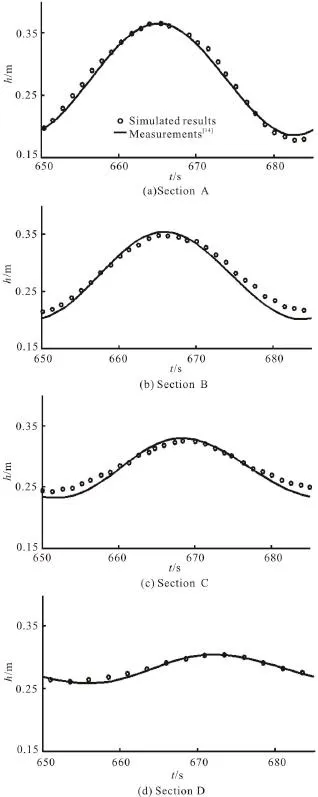
Fig. 7 Measured and simulated water elevation variations during one tidal cycle at middle points of four sections

The water elevations are measured at four sections (Sections A, B, C and D) as shown in Fig. 6 in the laboratory experiment. The numerical results are compared with the experimental data at the middle points of four sections A-B-C-D as shown in Fig. 7. It is demonstrated that the simulated results and the experimental data are in good agreement. The RMSE(root-mean-square error) values at Sections A, B, C and D are 0.007, 0.010, 0.010 and 0.007, respectively.Due to the wave attenuation inside the beach, the tidal range at Sections D is much smaller than those at other sections, which may be the reason why the RMSE value at Sections D is lower than those at Sections B and C.

In the simulation results, the tidal range on the beach face (Section A) is 0.175 m, which is almost the same as that in the surface water. It decreases with the increase of the distance away from the beach face. The tidal ranges are 0.158 m, 0.100 m, and 0.005 m at Section B, Section C and Section D, respectively. It indicates that the tidal wave attenuation occurs under the sandy beach. The ratio of the tidal range at Section B to that at Section A is 90.3%, while such ratios are 57.1% at Section C and 28.6% at Section D. As the tidal wave propagates inside the beach, its energy is reduced. The extent of the tidal wave attenuation is proportional to its propagation distance.

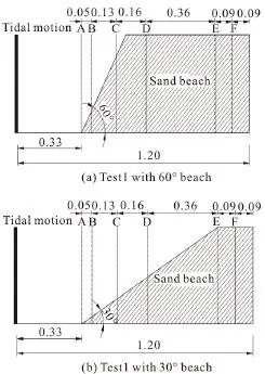
Fig. 8 Sketch of the tests investigating the tide-induced groundwater table fluctuation under sloping beaches (m)

The rectangular beach rarely exists in reality. To investigate the tide-induced groundwater table fluctuation under beaches with different slopes, two tests with sloping beaches are studied. A sketch of these two tests is shown in Fig. 8. Test 1 has a beach slope of 60°, and the beach slope in Test 2 is 30°. The simulated water elevation variations during one tidal cycle at middle points of A-B-C-D sections in Test 1,

Test 2 and under the rectangle beach are shown in Fig.9. At Section A, occupied by the surface water, the patterns of the flow in all three cases are the same.The surface water flow still exists in both sloping beaches at Sections B and C, while the tidal wave attenuation occurs in the rectangular beach. Large deviations appear at Section D, which is completely inside the beach in Test 1 and partially covered by the surface water in Test 2. The ratio of the tidal range at Section D in Test 1 to that at Section A is 45.7%,which is larger than that under the rectangular beach(28.6%). In Test 1, the distance between Section D and the beach face is less than 0.155 m, while it is 0.335 m under the rectangular beach. The longer distance would result in a more significant tidal wave attenuation.

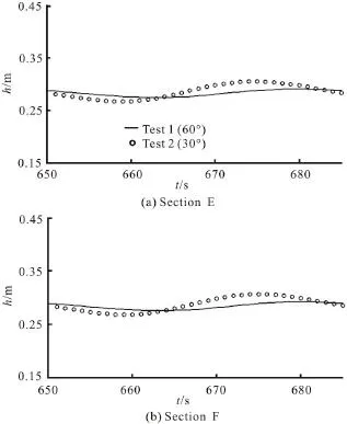
Fig. 10 Simulated water elevation variations during one tidal cycle at middle points of E-F sections with different beach slopes

Results of the groundwater fluctuation at Section E and Section F in Test 1 and Test 2 are shown in Fig.10. In both tests, the tidal wave attenuation is clearly seen at these sections. The tidal ranges at Section E and Section F are 0.016 m and 0.014 m, respectively in Test 1, and they are 0.043 m and 0.038 m in Test 2.The distances between Section E and Section F are the same in these two tests, but the tidal wave attenuation in Test 1 is much more significant than that in Test 2.The groundwater wave propagation is strongly affected by the beach slope. The larger the beach slope, the more intense the wave attenuation will be.

2.3 Wave setup due to the coastal barrier

The wave setup is a coastal phenomenon due to the transfer of the wave momentum to the underlying water column during the wave breaking process in the coastal area. This process leads to the transient rise and fall of the mean water level in the surf zone. It is an important issue in the design aspects of coastal and nearshore structures, where significant flooding and oscillating water levels can pose a significant threat to the long term stability of these structures. In the nearshore, where waves lose their stability and start to break, running up and down on the beach surface, a certain amount of water seeps into the permeable beach, generating a complex circulation in the porous medium. Associated with the wave breaking, the wave-induced groundwater flow in coastal aquifers is complicated and difficult to predict. Horn et al.[25]designed an experiment to simulate a coastal barrier dividing the ocean from a relatively constant back beach water level, and the wave setup level due to the coastal barrier was measured. Based on the experimental data, Bakhtyar et al.[15]coupled a hydrodynamic model to a groundwater flow model SEAWAT to simulate the wave-induced water table fluctuations.In his method, the groundwater flow is driven by a temporally-varying hydraulic head at the beach face computed by the hydrodynamic model of the surface water. In the present study, four tests of wave setup along a sloping beach is calculated by the fully integrated NHWAVE model, and the results are compared with the experimental data and the simulation results reported in previous studies. A sketch of the study domain is shown in Fig. 11. The waves are incident from the left boundary. The beach aquifer is 5.3 m long with a slope of 1:7.6. The mean water depth is 0.5 m for the free surface water. The grid size in the simulation is 0.003 m, and ten layers are employed in the vertical direction, and both the groundwater and surface water domains are discretized. The wave amplitude and period are 0.008 m and 2.5 s, respectively. The time step is determined in every calculation interval according to the CFL condition. Both fine and coarse sands are used to represent the beach sediment. The initial water elevation for the surface water has the same value as the mean water depth of 0.5 m in four tests, while the initial groundwater tables are different. Other parameters are shown in Table 1.

Figures 12(a)-12(d) show the comparisons of the present simulation results, the measured data in experiment[25], and the pervious simulation results[15]in four tests. Figure 12(a) displays the results of the wave setup on the fine sand beach when the initial groundwater table is identical to the mean water depth(Test 1). The model presented in this study gives results in better agreement with the measured wave setup in the surf zone than those reported in Ref. [15],although the groundwater table seems to be slightly overestimated. Similar results are shown in Fig. 12(b),where the initial groundwater table inside the fine sand beach is lower than the mean water depth (Test 2). Figure 12(c) shows the results of the wave setup on the coarse sand beach when the initial groundwater table is identical to the mean water depth (Test 3). The measured and simulated data of both the surface water and the groundwater are in reasonably good agreement. In Fig. 12(d) where the initial groundwater table inside the coarse sand beach is lower than the mean water depth (Test 4), a similar pattern of measured and simulated data can be observed. These results show that the modified NHWAVE model presented here could reproduce the wave setup and the groundwater table variation correctly.

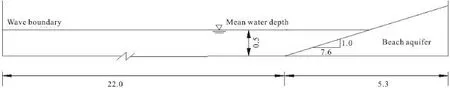
Fig. 11 Sketch of the study domain with free surface water and beach aquifer (m)

Fig. 12 Comparisons of measured and simulated wave setup levels (line: Simulated data in the present paper; circles: Measured data in laboratory experiment[25], dash line: Simulated data in Bakhtyar et al.[15], bold line: Beach face)

Fig. 13 Comparison of wave setups in impermeable and permeable beaches in Test 3

Through the comparisons between Test 1 and Test 3, and between Test 2 and Test 4, it is shown that the spatial change of the wave setup levels in the beach is larger in the fine sand than in the coarse sand.The wave setup level decreases from the beach face toward the inland area. The aquifer properties, such as the porosity and the hydraulic conductivity, have a great influence on the wave propagation in the permeable beach. The initial elevation difference of the surface water and the groundwater also affects thewave dynamics in the groundwater. Larger water elevation variation drives more water infiltration from the surface to the beach aquifer, which increases the wave setup level on the beach face. The largest discrepancy between the simulations in this paper and the experimental measurements appears at the location near the beach face on the fine sand beach. It might be caused by neglecting the capillarity effect in the model, which becomes important for the water infiltration in the porous media with a low porosity.

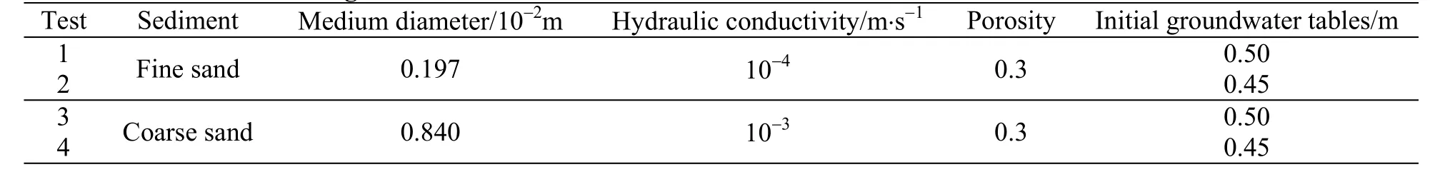
Table 1 Characteristics of groundwater conditions

In order to see the effect of the permeability of the beach on the surface water, the flow field of the surface water on an impermeable sandy beach is simulated. Other parameters are kept the same as in Test 3. As shown in Fig. 13, the wave setup level undergoes a significant change on an impermeable beach. At the pointx= 25.5 m , the difference of the wave setup levels is between these two cases. The wave setup level on the impermeable beach is much larger than that on the permeable beach. The wave runup on the impermeable beach face is also more intense. These results indicate that the permeability of the beach is an important factor influencing the hydrodynamics in the coastal zone, and the interactions between the surface water and the groundwater should be considered in the study of coastal hydrodynamics.

3. Conclusions

Based on the NHWAVE model, a fully integrated three-dimensional non-hydrostatic model is developed to simulate the interactions between the surface water and the groundwater affected by tides or waves in coastal areas. With the model, both the surface water flow and the groundwater flow are calculated based on the well-balanced VRANS equations. The spatially varying porosity and hydraulic conductivity are used to identify the domains for the surface water and the groundwater.

The model is calibrated and validated by a series of laboratory measurements, involving the tide propagation through a sandy embankment, the tideinduced groundwater table fluctuation in a sandy beach, and the wave setup level in a sloping sandy beach. The simulation results show that the model is capable of simulating both the tide driven and wave driven groundwater table fluctuations in coastal areas,as well as the wave setup level in sloping permeable beaches.

Through the numerical benchmarks, the dynamic interactions between the surface water and the groundwater are analyzed and the influencing factors on the groundwater table fluctuations are discussed.The phase lag between the surface water elevation and the groundwater table fluctuation is mainly influenced by the hydraulic conductivity of the porous media.With a larger hydraulic conductivity, the phases of the groundwater and the surface water in the coastal area are closer to each other. The wave attenuation in the groundwater is proportional to its propagation distance inside the permeable sandy beach, and the amplitude of the groundwater table fluctuation decreases faster with a larger beach slope. The wave setup level in the surf zone is larger on an impermeable beach. The spatial variation of the wave setup level in the beach is larger in the fine sand than in the coarse sand.

Results in this paper indicate that the permeability of the beach is an important factor influencing the hydrodynamics in the coastal zone, and the interactions between the surface water and the groundwater should be considered in related studies. The fully integrated surface water and groundwater model proposed in this paper can be used to study the dynamics and the interactions between the surface water and the groundwater in coastal areas.

[1] Liu Y., Shang S. H., Mao X. M. Tidal effects on groundwater dynamics in coastal aquifer under different beach slopes [J].Journal of Hydrodynamics, 2012, 24(1):97-106.

[2] Pauw P. S., Oude Essink G. H. P., Leijnse A. et al. Regional scale impact of tidal forcing on groundwater flow in unconfined coastal aquifers [J].Journal of Hydrology,2014, 517(9): 269-283.

[3] Lee E., Hyun Y., Lee K. K. Sea level periodic change and its impact on submarine groundwater discharge rate in coastal aquifer [J].Estuarine, Coastal and Shelf Science,2013, 121-122(4): 51-60.

[4] Post V. E. A. A new package for simulating periodic boundary conditions in MODFLOW and SEAWAT [J].Computers and Geosciences, 2011, 37(11): 1843-1849.

[5] Li L., Barry D. A., Cunningham C. et al. A two-dimensional analytical solution of groundwater responses to tidal loading in an estuary and ocean [J].Advances in Water Resources, 2000, 23(8): 825-833.

[6] Bakhtyar R., Barry D. A., Brovelli A. Numerical experi-ments on interactions between wave motion and variabledensity coastal aquifers [J].Coastal Engineering, 2012,60(2): 95-108.

[7] Geng X., Boufadel M. C., Xia Y. et al. Numerical study of wave effects on groundwater flow and solute transport in a laboratory beach [J].Journal of Contaminant Hydrology,2014, 165(9): 37-52.

[8] Li L., Barry D. A., Pattiaratchi C. B. et al. BeachWin:modelling groundwater effects on swash sediment transport and beach profile changes [J].Environmental Modelling and Software, 2002, 17(3): 313-320.

[9] Yang J., Graf T., Herold M. et al. Modelling the effects of tides and storm surges on coastal aquifers using a coupled surface-subsurface approach [J].Journal of Contaminant Hydrology, 2013, 149(6): 61-75.

[10] Liang D., Falconer R. A., Lin B. Coupling surface and subsurface flows in a depth averaged flood wave model [J].Journal of Hydrology, 2007, 337(1-2): 147-158.

[11] Castro-Orgaz O., Giraldez J. V. Steady-state water table height estimations with an improved pseudo-two-dimensional Dupuit-Forchheimer type model [J].Journal of Hydrology, 2012, 438-439(5): 194-202.

[12] Yuan D., Lin B., Falconer R. Simulating moving boundary using a linked groundwater and surface water flow model[J].Journal of Hydrology, 2008, 349(3-4): 524-535.

[13] Kong J., Xin P., Song Z. et al. A new model for coupling surface and subsurface water flows: With an application to a lagoon [J].Journal of Hydrology, 2010, 390(1-2):116-120.

[14] Yuan D., Lin B. Modelling coastal ground- and surfacewater interactions using an integrated approach [J].Hydrological Processes, 2009, 23(19): 2804-2817.

[15] Bakhtyar R., Brovelli A., Barry D. A. et al. Wave-induced water table fluctuations, sediment transport and beach profile change: Modeling and comparison with large-scale laboratory experiments [J].Coastal Engineering, 2011,58(1): 103-118.

[16] Ma G., Shi F., Kirby J. T. Shock-capturing non-hydrostatic model for fully dispersive surface wave processes [J].Ocean Model, 2012, 43-44(22-35): 22-35.

[17]Ma G., Kirby J. T., Su S. F. et al. Numerical study of turbulence and wave damping induced by vegetation canopies [J].Coastal Engineering, 2013, 80(4): 68-78.

[18] Ma G., Kirby J. T., Shi F. Numerical simulation of tsunami waves generated by deformable submarine landslides[J].Ocean Model, 2013, 69(3): 146-165.

[19] Ma G., Chou Y. J., Shi F. A wave-resolving model for nearshore suspended sediment transport [J].Ocean Model,2014, 77(5): 33-49.

[20] Ma G., Shi F., Hsiao S. et al. Non-hydrostatic modeling of wave interactions with porous structures [J].Coastal Engineering, 2014, 91(9): 84-98.

[21] Ma G., Su S., Liu S. et al. Numerical simulation of infragravity waves in fringing reefs using a shock-capturing non-hydrostatic model [J].Ocean Engineering, 2014,85(3): 54-64.

[22] Jesus M., Lara J. L., Losada I. J. Three-dimensional interaction of waves and porous coastal structures, Part I:Numerical model formulation [J].Coastal Engineering,2012, 64(2): 57-72.

[23] Kherbache K., Chesneau X., Zeghmati B. et al. The effects of step inclination and air injection on the water flow in a stepped spillway: A numerical study [J].Journal of Hydrodynamics, 2017, 29(2): 322-331.

[24] Ebrahimi K. Development of an integrated free surface and groundwater flow model [D]. Doctoral Thesis, Cardiff,UK: Cardiff University, 2004.

[25] Horn D. P., Baldock T. E., Li L. The influence of groundwater on profile evolution of fine and coarse sand beaches[C].Proceedings of Coastal Sediments 07, New Orleans,USA, 2007, 506-519.