Changhong Hu, Cheng Liu

Research Institute for Applied Mechanics, Kyushu University, Fukuoka, Japan

Introduction

Prediction of strongly nonlinear interaction between violent free surface flow and floating body is important in many ocean and offshore engineering applications. However, numerical simulation of such wave-body interaction problem has many difficulties since turbulent phenomenon, wave breaking, violent body motion and free surface impact should be properly considered.

Accurate numerical simulation of turbulent free surface flows requires very high spatial resolution for the regions with small-scale fluid structures or with large gradients of flow variables. However, even by using a modern HPC, direct numerical simulation(DNS) of a fully developed macro-scale turbulent flow is still a big challenge[1]. Due to the fractal nature of the turbulence phenomenon, it is reasonable to use different grid resolutions to capture the flow structure of different scales in numerical simulations. This provides the motivation for us to develop an efficient adaptive mesh solver for simulation of violent free surface flows.

The CFD solver we are now developing is a blocked AMR solver, which is designed for the use in a distributed memory parallel computer system. High parallelization efficiency of the AMR solver is the key point of our concern. Main features of our solver are summarized as follows. First, we extend the interface capturing method including THINC[2]and VOF[3]schemes for sharp representation of moving distorted interfaces. Second, to preserve the flux conservation, a prolongation approach by using CIP method is proposed for filling the fluxes in newly created cells.Our conservative prolongation treatment is motivated by Chen et al.[4], in which the corner point value (PV)and volume integrated average (VIA) are used to build the multi-dimensional interpolation. In our method,surface integrated average (SIA) and VIA are used to complete the prolongation with the assistant of multi-dimensional Lagrange polynomial interpolation(LPI). Third, a fast algorithm for generating the coefficient matrix of elliptic operator, which is based on unstructured mesh topology, is proposed. Different from other adaptive methods, our algorithm is specially designed for blocked adaptive meshes, in which the matrix assembling occupies a very small portion of the total running time.

Our AMR framework has been tested for solving compressible Euler equation[5], compressible multimedium flows[6]and incompressible flows with immersed boundary (IB) method[7]. In this paper, we extend the AMR framework to the simulation of violent free surface flows.

1. Mathmatical model

1.1 Governing equations

Incompressible flow is assumed and the follo-wing integral form of the incompressible Navier-Stokes equation is used.

where n is the unit normal vector of the surface S,Ω is the control volume enclosed by S, u and p indicate the velocity vector and pressure, respectively.τ= μ [▽ u + (▽ u )T] is the shear stress tensor. f stands for the body force, such as the gravity force. A fractional step method[8]with second order accuracy is adopted for decoupling the pressure and velocity. The free surface flow is treated as a multiphase problem,which includes a liquid phase and a gas phase. To recognize different phases we define a volume fraction Γ, of which =1Γ indicates the water phase, =0Γ the air phase. The CIP-CSL2[9]with third order accuracy in spatial reconstruction is applied for discretization of advection term. Diffusion term and pressure term are treated by standard FVM.

1.2 Interface capturing method

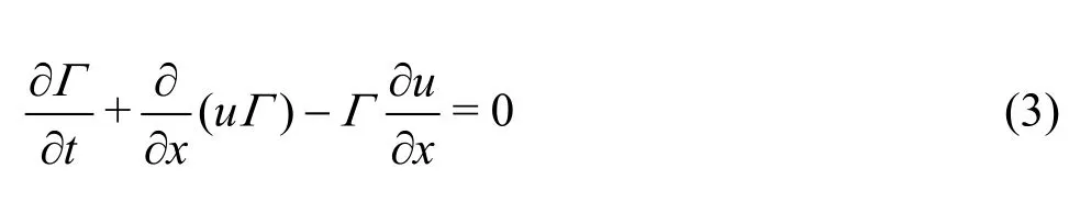
For applying the THINC/SW scheme, the following 1-D transport equation on the volume fraction Γ is used.

For multi-dimensional problems, a simple dimension-by-dimension approach proposed by Xiao et al.[10]is adopted. The approximated value of cell-average of Γ( x , t ) over the cell of [ xi-1/2, xi+1/2]can be calculated as follows

The piecewise modified hyperbolic tangent function( x ) is used to approximate the profile inside the cell

The parameters α, δ and β are defined to control the shape of the hyperbolic tangent function( x) and to obtain a better approximation of the sharp transition of the volume function inside a cell.Details can be found in Ref. [10].1.3 Adaptive mesh refinement

A blocked structured adaptive mesh with semioverlapped grid topology, which is shown in Fig. 1, is developed as the present AMR treatment. The basic unit for manipulation is the block as shown in Fig.1(a). The problem is discretized on a series of blockL=0,1… ,L max), in which B is the coarsest level and the level of +1L is finer than the level of L by a factor of 2. To efficiently manage the topology of the block, the octree-based hierarchical data structure is used (Fig. 1(b)), in which {LBΩ∈｝,Ω= ΩL∪ΩB, where Ω is the set of all nodes, ΩLandBΩ are the set of leaf nodes and branch nodes,respectively. The numerical solution is advanced onlyIt is noted that no memory space is allocated for the nodes marked by blank circle as in Fig. 1(b). The Peano and Hilbert space-filling curves[11]are generated based on the octree to realize a dynamical loading balance among the processors.

Fig. 1 (Color online) 3-D adaptive mesh and its representations as an octree

2. Numerical result

2.1 Numerical test on interface capturing method

This numerical example is performed on a benchmark case for validation of the interface capturing scheme. A circle interface with initial radius of R = 0.2 at （0,-0.25） is evolved with a 2-D velocity field represented by the following equation, u=-s in(π x ) cos(π y) and v = - c os(πx ) sin(πy). The computations are carried out using AMR with CFL number of 0.2. The volume fraction field and the

adaptive mesh blocks are plotted together in Fig. 2. It can be seen that the mesh around the regions of the moving interface is sufficiently refined during the computation. To check the conservative property of the two interface capturing methods (THINC,THINC/SW), we define the1Lerror of the total mass.

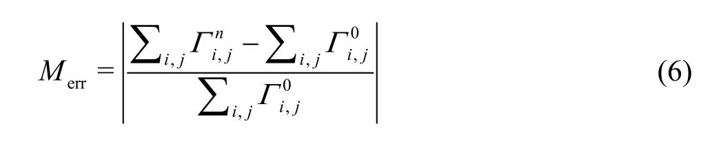
whereindicates the total mass of the initial VOF field andrepresents the final total mass. The1Lerrors at =14tare shown in Table 1.THINC/SW scheme shows better performance than THINC scheme for our AMR solver.

Table 1 1L errors for single-vortex shearing flow test

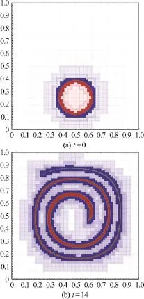
Fig. 2 (Color online) Single-vortex shearing flow test with THINC method, adaptive mesh level of 4-7

The next advection test is performed to validate the AMR solver in preserving the interface shape and the total mass for 3-D problems. The VOF field is initialized by a sphere with radius of 0.15 located at(0.35,0.35,0.35) in a computational domain of a unit cube. The incompressible velocity field updates as in reference[12]. Figure 3(a) shows the instantaneous iso-surface (Γ = 0.5) of the volume fraction field.Three levels adaptive mesh (level 4-7) is used, as shown in Fig. 3(b). During the simulation, all the blocks containing interfacial cells are marked to be refined, which means the regions where conservative errors become large are always covered by finest mesh. The total mass error1Lunder different mesh resolution is listed in Table 2. It is found that same accuracy can be achieved with much less grid number by using AMR method that that by using uniform mesh.

Fig. 3 (Color online) Numerical test on a 3-D advection problem, adaptive mesh level of 4-7

2.2 Capillary wave test

The adaptive two-phase flow solver is validated by a classical benchmark test, a small-amplitude capillary wave problem (with gravity). For the present capillary wave problem, the free surface driven by the gravity oscillates periodically. It can be expected thatunder the viscous effect, the amplitude of wave oscillation is damped with time. In the numerical simulation the computational domain is set as x ∈ [-0 .5λ, 0 .5λ] and y ∈ [-1 .5λ,1 . 5λ]. Here λ denotes the wavelength of the perturbation. The initial wave profile is defined as H( x, t0) = A0cos(k x),where A0= λ / 1 00 is the perturbation amplitude,k=2π/λ is the wave number.

Table 2 1L error at =t T

In Fig. 4, computed relative maximum interface height as a function of time is compared with the solution by the theoretical analysis[13]. I can be seen that the present computation agrees perfectly to the theory.

Fig. 4 (Color online) Ev ol ution of t he a mplitudes of the g ravity waveprofileasafunctionofnon-dimensionaltime, = 10, = 1, g =50

2.3 Numerical test of breaking wave

Finally, numerical simulation of a wave-breaking problem is carried out by the AMR solver. The splash-up mechanism of wave-breaking deserves fully investigation because it plays a significant role in the dissipation of the wave energy. It is challenging CFD topic for conventional Cartesian grid method since a large amount of bubbles are entrapped in the water and also many small droplets exist. Present AMR solver provides an efficient way to treat these bubbles/droplets by local refinement.

The numerical test starts from a sinusoid wave with very large wave steepness (H /λ = 0.13). The initial wave will soon become instable and finally wave breaking appears. The computational domain is x, z ∈ [-0 .5λ, 0 .5λ], y ∈ [-0 .125λ,0.125λ], where λ=0.2 m is the wavelength of the initial free surface.Since the periodic boundary condition is specified on the left and right boundary, the wave that moves out of the right boundary re-enters to the left side. The density and dynamic viscosity for the two phases(water and air) are ρwater=998 kg/m3, μwater=1.0×10-3Pa· s , ρ=1.25 kg/m3and μ =1.8×

airair10-5Pa· s . The initial velocity field ( u, w ) and

00wave height0(())h x are given by linear wave theory as follows:

where =2/kLπ is the wave number, d the water depth, H the wave height. The refinement level from 2 to 5 is used where the coarsest and the finest level corresponds to a uniform mesh with 64×32×64 and 512×256×512 grid number covering the whole computation domain, respectively. Each block is filled with a 8×8×8 uniform grid. During the simulation, the cells related to the free surface are always covered by finest blocks.

Present parallel computation is carried out in a HPC cluster system with 20 physical cores (Intel Xeon E5-4627, 3.4GHz). A high performance message passing library (Open MPI) is applied for data communication among processors. The derived pressure Poisson equation is solved by third-party mathematical libraries Hypre[14]and PETSc[15].

The free surface profiles evolved with time are given in Figs. 5(a)-5(j). After the computation starts,the wave steepen increases gradually with the wave propagation. Once the front of the wave crest becomes vertical (Fig. 5(c)), a thin jet is observed which falls down and hits the water surface (Fig. 5(d)). Air entrapment by the jet (air pocket) is observed. A secondary plunging breaking wave is then formed (Fig.5(e)), in which splashes spill down to the free surface again and generate turbulent air/water mixing flows(Fig. 5(g)). The kinematics and dynamics of overturning motion are well reproduced by present AMR solver, and the general trend of the flow dynamics is well simulated.

Fig. 5 (Color online) Instantaneous free surface profiles at different time

3. Conclusion

In this paper, we present our new developments on the AMR solver for simulating violent free surface flows. The CIP method is applied to the flow solver and THINC/SW is implemented as the interface capturing scheme. The linear solver is redesigned and modified to satisfy the requirement of the AMR mesh topology. Several fundamental validation tests have been carried out showing that the present numerical approach is efficient and accurate for incompressible free surface flows. Numerical simulation of a wave breaking problem has also been carried out. The numerical result shows that very fine flow structures,e.g., splashing, droplet, and air entrapment can be successively simulated by the AMR approach.

[1] Scardovelli R., Zaleski S. Direct numerical simulation of free-surface and interfacial flow [J].Annual Review of Fluid Mechanics, 1999, 31(1): 567-603.

[2] Xiao F., Ii S., Chen C. Revisit to the THINC scheme: A simple algebraic VOF algorithm [J].Journal of Computational Physics, 2011, 230(19): 7086-7092.

[3] Hirt C. W., Nichols B. D. Volume of fluid (VOF) method for the dynamics of free boundaries [J].Journal of Computational Physics, 1981, 39(1): 201-225.

[4] Chen C., Xiao F., Li X. An adaptive multimoment global model on a cubed sphere [J].Monthly Weather Review,2011, 139(2): 523-548.

[5] Liu C., Hu C. An immersed boundary solver for inviscid compressible flows [J].International Journal for Numerical Methods in Fluids, 2017, 85(11): 619-640.

[6] Liu C., Hu C. Adaptive THINC-GFM for compressible multi-medium flows [J].Journal of Computational Physics, 2017, 342: 43-65.

[7] Liu C., Hu C. An adaptive multi-moment FVM approach for incompressible flows [J].Journal of Computational Physics, 2018, 359: 239-262.

[8] Min C., Gibou F. A second order accurate projection method for the incompressible Navier-Stokes equations on non-graded adaptive grids [J].Journal of Computational Physics, 2006, 219(2): 912-929.

[9] Xiao F., Ikebata A., Hasegawa T. Numerical simulations of free-interface fluids by a multi-integrated moment method [J].Computers and structures, 2005, 83(6):409-423.

[10] Xiao F., Honma Y., Kono T. A simple algebraic interface capturing scheme using hyperbolic tangent function [J].International Journal for Numerical Methods in Fluids,2005, 48(9): 1023-1040.

[11] MacNeice P., Olson K. M., Mobarry C. et al. PARAMESH:A parallel adaptive mesh refinement community toolkit [J].Computer Physics Communications, 2000, 126(3):330-354.

[12] Xiao F., Ii S., Chen C. Revisit to the THINC scheme: A simple algebraic VOF algorithm [J].Journal of Computational Physics, 2011, 230(19): 7086-7092.

[13] Prosperetti A. Motion of two superposed viscous fluids [J].Physics of Fluids, 1981, 24(7): 1217-1223.

[14] Falgout R. D., Yang U. M. Hypre: A library of high performance preconditioners [C].International Conference on Computational Science, Amsterdam, The Netherlands,2002, 632-641.

[15] Balay S., Brown J., Buschelman K. et al. PETSc user’s manual revision 3.4 [R]. Argonne, IL, USA: Computer Science Division,Argonne National Laboratory, 2012.