Touvia Miloh , Ioannis K. Chatjigeorgiou

1. Faculty of Engineering, Tel Aviv University, Ramat Aviv, Israel

2. School of Naval Architecture and Marine Engineering, National Technical University of Athens, Athens,Greece

Introduction

Ellipsoidal geometries in fields governed by anisotropic potentials have many important applications in science and modern technology. To list a few, reference is made to electrostatics, electromagnetics, acoustic scattering, brain imagining, tumor growth simulation and apparently, hydrodynamics. In relevant applications the solution of the field equation is described by ellipsoidal harmonics, first obtained by Gabriel Lamé in 1837. Lamé in his celebrated paper on temperature distribution in an ellipsoid[1]has managed to separate the Laplace equation in a coordinate system consisting of second degree surfaces.This system is known today as the ellipsoidal system.In fact, Lamé himself proposed the classification of the solutions of the obtained ordinary differential equation in four classes having a particular structure and he produced the first few solutions in each class.Products of these functions generate the ellipsoidal harmonics.

It is worth mentioning that this particular analysis by Lamé, gave rise to what we refer today as the theory of curvilinear coordinates, a theory also developed by Lamé[2]. Many famous mathematicians produced excellent results on Lamé functions and ellipsoidal harmonics during the whole of 19th century. A fairly complete collection of these results as well as historical notes can be found in the recently published book of Dassios[3].

All these efforts resulted in a well-defined theoretical structure for dealing with boundary value problems in ellipsoidal geometry, which, unfortunately, cannot be very effective without the use of computational techniques. Some attempts to produce numerical solutions of Lamé functions, and therefore of ellipsoidal harmonics, appear in the literature in the early 1960’s. In that context, reference is made to the books of Arscott and Khabaza[4]and Arscott[5].

In hydrodynamics, the quest for analytical solutions for hydrodynamic boundary value problems in the Laplace domain involving ellipsoidal geometries is indeed a great challenge. To the authors’ best knowledge, the only attempts in that respect were those due to Havelock[6]and Miloh[7]. Havelock[6]considered the wave resistance (only) problem of ellipsoidal forms and provided rather simplified formulae for its calculation. Havelock’s[6]theory didn’t employ the actual ellipsoidal harmonics, i.e.Lamé functions, whilst no numerical calculations were performed. Miloh[7]employed the Lagally theorem[8-10]to analyze the general maneuvering of ellipsoids. The study indeed relied on the ellipsoidal harmonics but,again no numerical implementation was performed.

The analytical approach to the solution for the hydrodynamic diffraction problem by immersed ellipsoids involves two major difficulties. The first is associated with the derivation of closed forms that satisfy the conditions of the governing boundary value problem and the second is the numerical calculation of the ellipsoidal harmonics of both kinds. In fact, the latter must be obtained for arbitrary large degrees and orders to allow achieving convergent results. However,nearly all the existing studies which provide formulas for calculating the Lamé functions stop at degree n = 3 [3]. Only recently Dassios and Satrazemi[11]provided formulas up to degree =7n. Even these formulas however require numerical solution.

In the present contribution we have undertaken both tasks, i.e., the two major difficulties mentioned in the previous paragraph. In particular, we developed a robust and efficient algorithm that was accordingly implemented into a computer code that is able to calculate the Lamé functions of both kinds and for arbitrary large degrees and orders. In addition, the concerned methodology can properly calculate the orthogonality constants by employing the general orthogonality relation satisfied by the Lamé functions of the first kind. The mathematics behind the numerical algorithm and the computer code is that of the general theory of Lamé functions that can be found in the book of Dassios[3].

As far as the analytic solutions of the hydrodynamic problems considered at present are concerned,namely the attraction force and the added mass for an ellipsoid moving steadily in parallel and close to a rigid wall as well as the ship crossing encounter problem, they were obtained by applying the method of ultimate image singularities of tri-axial ellipsoids which were rigorously derived by Miloh[12].

1. A steadily translating tri-axial ellipsoid close to a rigid wall

1.1 The ellipsoidal coordinate system

Ellipsoidal coordinates (,,)λ μ ν are defined relative to the basic ellipsoid

where

The three surfaces λ=constant (ellipsoids),μ=constant(hyperboloids of one sheet), ν=constant (hyperboloids of two sheets) form a triply orthogonal coordinate system in space. For ξ=λ,μ or ν, these surfaces satisfy the equation

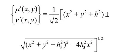
The ellipsoids λ =constant are confocal with that for λ=a1. The limiting member of this family, given by λ=h2, is the area of thez-plane bounded by the“focal ellipse”

The roots of Eq. (4) are chosen so that

1.2 The Green’s functions and its multipoles

We define now a Cartesian (,,)x y zcoordinate system fixed on the centre of the solid. Thex-axis is the longitudinal axis of the ellipsoid while they-axis is pointing toward and normally to the wall. The Green’s function that satisfies the Laplace equation and the zero-velocity condition on the wall is

wheredis the distance between the centre of the ellipsoid and the rigid wall. Accordingly, the multipoles of the Green’s function are obtained by using Miloh’s theorem on even exterior ellipsoidal harmonics[12]. It should be noted that only the even harmonics are retained as the problem is symmetric inzand hence only the Lamé functions which are even inzmust be considered. The Lamé functions which are even inzare those of classes Kand L. Thus we have

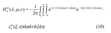
where0Sis the area of the focal ellipse (4). Using the Miloh’s theorem[12], Eq. (7) yields

wheredenotes the multipoles of the Green’s function,,are the Lamé functions of the first and the second kind, of ordermand degreen,whiledenotes the source distribution over the fundamental ellipse (4), given by[12]

where

The integral in Eq. (8) will be denoted by(λ, μ ,ν) . Taking the Fourier Transform of the last component we obtain

Given that the extremes ofyin the fundamental ellipse are ±a2, the above formula is valid fory＜2d-a2

1.3 Expansion of regular terms in ellipsoidal harmonics

Let us further assume that the exponential term exp[τy+iτ(xc osφ +zsin φ )] is expanded using interior ellipsoidal harmonics according to

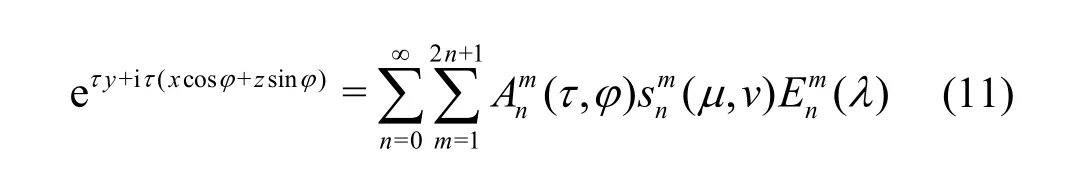
where (,)τ φ are coefficients to be determined. To obtain those coefficients, Eq. (11) is evaluated on the surface of the ellipsoid, defined at1=aλ which in turn allows us to exploit the fundamental relation of orthogonality[3]. Subsequently, the coefficients sought will be given by

whereare the normalization (orthogonality)constants and the integration is taken over the surface of the ellipsoidSa, while (x0,y0,z0) denote the Cartesian representation of that surface evaluated by Eq. (2) using λ=a1.

Introducing Eqs. (12), (13) into the regular terms of Eq. (10) the latter can be written as

and the coefficientsare obtained by

where we let dS0=dξ d η and (x0,y0,z0) are understood as functions of (μ ,ν).

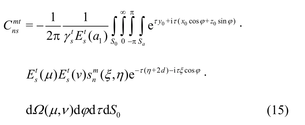
The Green’s function multipoles are now expressed by

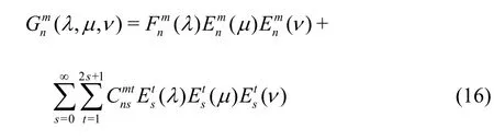
The coefficientscan be relatively simplified by calculating two of the involved integrals. One may use the following formulae

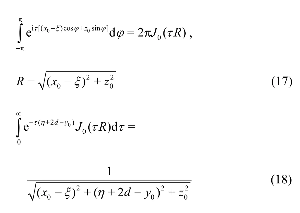
to yield

1.4 The velocity potential

The ellipsoid was assumed to translate steadily(alongx) close to a wall. Hence, the velocity potential will be composed by the equivalent uniform stream and the disturbance potential that is constructed in ellipsoidal harmonics using the multipole potentials of Eq. (16). In particular, it holds that

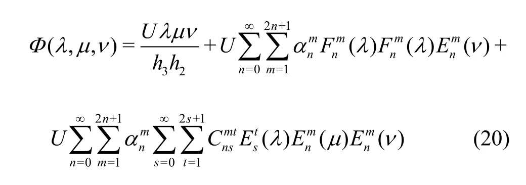
The unknown expansion coefficients αnmare to be determined. We note that these are dimensional and are expressed in length units. Again, the velocity potential must satisfy the Neumann condition on the surface of the ellipsoid, and in other words

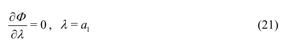
W 1e 1n oμtνe =t hEa t( μ1 )1E (ν )Thuafter introducing Eq. (20) into the boundary condition of Eq. (21)and making use of the orthogonality relation[3], the following linear system is derived

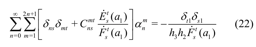
where δnsis the Kronecker’s delta function. Eq. (22)is to be solved in terms of the unknown expansion coefficients. Having calculated the latter, the total velocity potential is immediately derived through Eq. (20). In fact, the derivation ofcompletes the solution of the problem. Clearly, the linear system (22)must be truncated to a sufficient maximum degree to be solved using standard matrix techniques.

1.5 The attraction force

“Attraction force” is designated the force that is applied normal to the direction of motion, which thrusts the body toward the rigid wall. The disturbance here, has a more complicated structure than the usual flow lines that occur when the body moves steadily(or is subjected to a uniform stream) in an unbounded mass of liquid. The attraction force, coinedyF, is convenient to be calculated by the steady Lagally theorem[8-10], namely

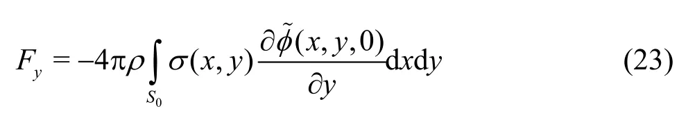
where σ(x,y) is the source distribution on the fundamental ellipse, while the integration is performed over the areaS0of that ellipse. In addition, φ~(x,y,0) denotes the regular term of the disturbance potential evaluated explicitly on the fundamental ellipse lettingz= 0 The source distribution is obtained by

while the regular term of the disturbance potential is obtained using Eq. (6) as

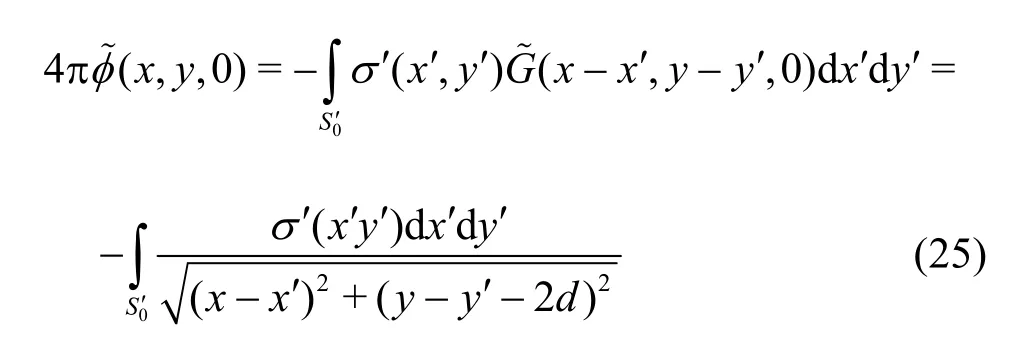
wheredenotes the second term of the right-hand side of Eq. (6). Assuming finally unit velocityU= -1, the normalized attraction force will be given by

The phenomenon is symmetric inz. Therefore, the source distribution (24) should involve only the Lame functions which are even inz, namely the classes K and L.

1.6 Added mass in the direction of motion

The Taylor added mass theorem[13]requires that the added massMis given by

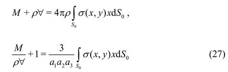
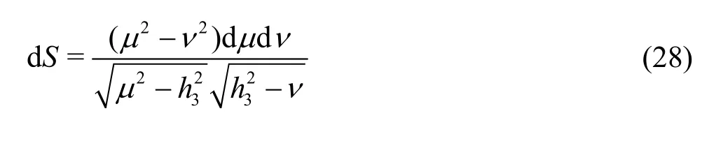
where the integration is performed over the area of the fundamental ellipse (4), in whichx= μ ν/h3and the differential area for λ=h2will read

The source distribution has been already given in Eq.(24) and we note that only the even system of singularities is considered given that the problem is symmetric inz. Eq. (27) in its extended form will read

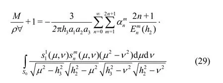
where(μ ,ν) =( μ)ν). The integral in Eq.(29) is evaluated by orthogonality and is equal to/ 2[3]. The final relation that provides the added mass is

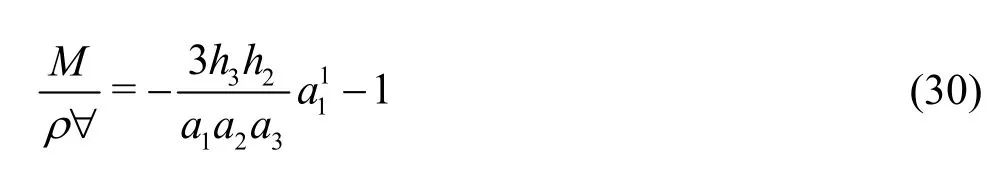
and it is clearly seen that depends on only one coefficient. The unbounded case away from the wall(d→∞) can be recovered usingHence, the asymptotic value ofMis

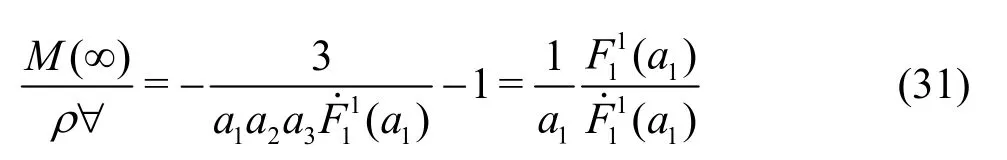
which can also be expressed in terms of elliptic integrals as given by Kochin et al.[14]and Lamb[15].Figures 1, 2 show some results for the attraction force and the added mass coefficients for the concerned mode of motion. It is clearly seen that the attraction force vanishes for large distances from the wall while the added-mass converges to the asymptotic value obtained by Eq. (31).

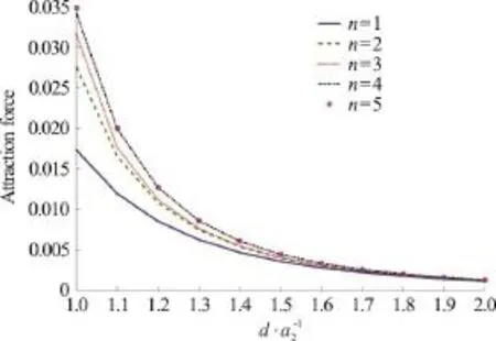
Fig. 1 (Color online) Attraction force acting on an ellipsoid 1 2 3 (a ,a ,a ) = (1,0.8,0.6) moving steadily close to a wall for increasing distance from it. The force has been normalized by 1 ρ a for unit velocity U

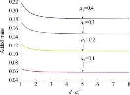
Fig. 2 (Color online) Added mass coefficients λ11=Mρ∀ for an ellipsoid ( a1 , a 2 )=(1,0.5) and several values of a3

2. Two ship encounter

Here we examine a common event that is always encountered during ship maneuvering operations,especially in ports, namely when two ships come across each other. In relevant situations, the forces exerted on ships, depending on the relative distances,the velocities and the direction of motions, may attract or repulse the ships. To analyze the phenomenon, we formulate the problem assuming significant simplifications and we approximate the ships by ellipsoidal geometries.

Fig. 3 Two ships encounter

We consider two ships maneuvering in a quiescent liquid in close proximity (Fig. 3) with two distinct steady velocitiesU1andU2with a relative course angle β. For simplicity we take the two ships to have the same geometry, represented by identical tri-axial ellipsoids, where the origin of the ship,expressed in an instantaneous system attached to the ship 1, isO2(X,Y). Thezcoordinate in the direction of gravity (directed into the fluid) is the same for both ships. Thus, the relation between the two Cartesian coordinate systems is simply given by

For the analysis that follows, we need to interchangeyandzin the equation of the ellipsoid (1)and the transformations between Cartesian and ellipsoidal coordinate systems (2), so that we will still havea1＞a2＞a3. The small semi-axis now is they-axis and all other parameters remain the same.

We assume that the draughts of the ships are larger than their beams. We also denote the induced source distribution on the fundamental “ellipse” of the ship 1 by σ1(x1, 0,z1) and the velocity potential enforced around ship 1 by the rectilinear motion of ship 2, by σ2(x1,y1,z1). Using further the steady Lagally theorem one can readily express the sway force and yawing moment exerted by ship 1 as

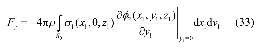
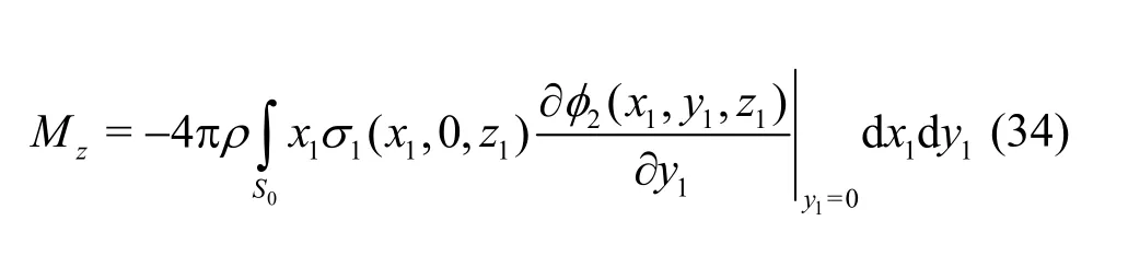
whereS0denotes the area of the fundamental ellipse(4). We further assumeU1=U2=U. The leading order source distribution σ1(x1, 0,z1) as provided by Miloh[12]is

C1(K) is literaryλ) evaluated on λ=a1. The factorKdenotes that the associated Lamé function is of class K. Eq. (36) enable us to express φ2(x1,y1,z1,X,Y,β) by virtue of Eqs. (32) as

where σ2(x2, 0,z2)is again obtained by Eq. (35).Taking the derivative of the above with respect toy1and evaluating ony1=0 we obtain

Introducing Eq. (38) into Eqs. (33), (34), one may calculate the sought sway force and yaw moment.

Fig. 4 Normalized force exerted by ship 1 as the two ships move rectilinearly in opposite directions (β =180°) .The ships have been approximated by tri-axial ellipsoidswith geometrical particulars 1 2 3 (a ,a ,a ) = (2,1,0.2) . Negative force indicates attraction (opposite direction of 1 y shown in Fig. 3) and positive force indicates repulsion

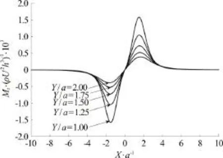
Fig. 5 Norm alized momen t e xerted by ship 1 as the two ships moverectilinearlyinoppositedirections (β= 180°).The ships have been approximated by tri-axial ellipsoids with geometrical particulars ( a1 , a2 , a 3 )=(2,1,0.2)

Numerical examples of the attraction-repulsion phenomenon that occurs during two-ship encounter are depicted in Figs. 4 and 5. In particular, two ellipsoidal ships were considered traveling in opposite directions with steady velocities until the meet each other. The beam to draught ratio, here denoted bya3/a2was assumed to be sufficiently small. Also, the spacing between the ships was assumed to be sufficiently large to avoid time-dependent source distributions which must be considered within ship 1 in the case of small spacing. Clearly, when the ships approach each other a repulsion force is applied and accordingly when the bows of the ships are hypothetically attached in the (x,z) plane yielding a separation distance between centres 2a1(note that they were considered identical), repulsion changes to attraction the maximum of which occurs when they-axes coincide. At that point the moment changes sign while when they-axes coincide the moment is zero. The above discussion agrees with the remarks made in the study of Yeung[16].

3. Conclusions

In the present study we addressed three crucial problems in marine hydrodynamics, namely the calculation of the attraction force and the added mass coefficients for an ellipsoid moving steadily close to a rigid wall and the ship crossing problem when two ships are moving steadily and relatively to each other and they are finally encountered. For the latter problem the two ships were assimilated by reference ellipsoids under the low Froude number assumption.The solutions were based on using linear potential theory and the method of ultimate image singularities for ellipsoidal harmonics developed by the senior author of this effort[12]. The numerical implementation was based on a newly developed numerical algorithm which is able to calculate the Lamé functions of arbitrary degree and order allowing thus the employment of a large number of ellipsoidal harmonics.

[1] Lamé G. Sur les surfaces isothermes dans les corps solides homogénes en équilibre de temperature [J].Journal de Mathématiques Pure et Appliquées, 1837, 2: 147-183.

[2] Lamé G. Leçons sur les coordonnées curvilignes et leurs diverses applications [M]. Paris, France: Mallet-Bechelier,1859.

[3] Dassios G. Ellipsoidal harmonics. Theory and applications [M]. Cambridge, UK: Cambridge University Press,2012.

[4] Arscott F. M., Khabaza I. M. Tables of Lamé polynomials [M]. Oxford, UK: Pergamon Press, 1962.

[5] Arscott F. M. Periodic differential equations. An introduction to Mathieu, Lamé and allied functions [M]. Oxford,UK: Pergamon Press, 1964.

[6] Havelock T. H. The wave resistance of an ellipsoid [J].Proceedings of the Royal Society of London, 1931, A132:480-486.

[7] Miloh T. Maneuvering hydrodynamics of ellipsoidal forms[J].Journal of Ship Research, 1977, 23(1): 66-75.

[8] Lagally M. Berechnung der krӓfte und momente, die strӧmende flüssigkeiten auf ihre begrenzung ausüben [J].Zeitschrift fur Angewandte Mathematik und Mechanik,1922, 2: 409-422.

[9] Landweber L., Yih C. S. Forces, moments and added masses for Rankine bodies [J].Journal of Fluid Mechanics, 1956, 1: 319-336.

[10] Landweber L., Miloh T. Unsteady lagally theorem for multipoles and deformable bodies [J].Journal of Fluid Mechanics, 1980, 96: 33-46.

[11] Dassios G., Satrazemi K. Lamé functions and ellipsoidal harmonics up to degree seven [J].International Journal of Special Functions and Applications, 2014, 2: 27-40.

[12] Miloh T. The ultimate image singularities for external ellipsoidal harmonics [J].SIAM Journal of Applied Mathematics, 1974, 26(2): 334-344.

[13] Taylor G. I. The forces on a body placed in a curved or converging stream of fluid [J].Proceedings of the Royal Society, 1928, A120: 260-283.

[14] Kochin N. E., Kibel I. A., Rose N. V. (Radok J. R. M Theoretical hydromechanics) [M]. New York, USA: Interscience Publishers, John Wiley and Sons, 1964.

[15] Lamb H. Hydrodynamics [M]. Cambridge, UK: Cambridge University Press, 1932.

[16] Yeung R. W. On the interaction of slender ships in shallow water [J].Journal of Fluid Mechanics, 1978, 85: 143-159.