Xiao-cui Wu (吴小翠), Yi-wei Wang (王一伟), Chen-guang Huang (黄晨光),

Zhi-qiang Hu 4(胡志强), Rui-wen Yi 4(衣瑞文)

1. Key Laboratory for Mechanics in Fluid Solid Coupling Systems, Institute of Mechanics, Chinese Academy of Sciences, Beijing 100190, China

2. School of Engineering Science, University of Chinese Academy of Sciences, Beijing 100049, China

3. Beijing Power Machinery Institute, Beijing 100074, China

4. Shenyang Institute of Automation, Chinese Academy of Sciences, Shenyang 110016, China

Introduction

The dynamic characteristics are an important factor in the surface vehicle design. This paper focuses on the wave making resistance and the lateral control maneuverability. With the development of the computational fluid dynamics, the Reynolds averaged Navier-Stokes (RANS) method with consideration of the fluid viscous effects for ship wave problems is used more extensively than the theoretical and experimental methods.

The blended-wing-body (BWB) is an appropriate candidate for the aircraft shape[1]. Remarkable performance improvements of the BWB are shown over the conventional baseline, including a 15% reduction in the takeoff weight and a 27% reduction in the fuel consumption per seat mile[2]. The aerodynamic characteristics were studied[3-4]. The effects of the spanwise distribution on the BWB aircraft aerodynamic efficiency and the effect of the taking-off, the landing and the heavey rain were simulated[5-6]. The coupled aeroelastic/flight dynamic stability and the gust response of a blended wing-body aircraft were also studied[7]. Because of its high lift to drag ratio and the large interior space, the BWB shape finds a certain application prospect for the surface vehicle, such as in the manta ray propulsion system[8-9]. A small, fast,lift-type vehicle was proposed based on the simulation of the manta ray[10-11]. The method for free-surface flows calculation are also discussed in Refs. [12-13].But for the industrial application of the vehicle, the wave making resistance and the lateral maneuvera-bility remain to be issues to explore. At present, the common shape of a ship is a slender hull. The frictional resistance is about 70%-80% of the total resistance, the viscous pressure resistance accounts for more than 10% of the total resistance, and the wave resistance component is very small in the case of a low speed. But in a high speed ship, the wave resistance will increase dramatically, reaching 40%-50% of the total resistance[14]. With the development of the ship industry, the research of the wave resistance has a practical application value.

In this paper, the dynamic characteristics of a small surface vehicle with a BWB shape are studied.The governing factors of the hydrodynamic characteristics are analyzed by the dimensional analysis method. The resistance and the control maneuverability characteristics are compared with those of the conventional ship. The implicit VOF method is adopted to simulate the wave resistance of the high speed BWB vehicle, and a semi-relative reference frame method is proposed to compute the hydrodynamic coefficients. The navigation speed, the drift angle and the rotating arm tank radius are computed to reveal the effect on the free surface hydrodynamic coefficients, to provide some reference for the simulation of the same type vehicle in the future.

1. Mathematical models

The governing equations are the RANS equations.

The continuity equation is

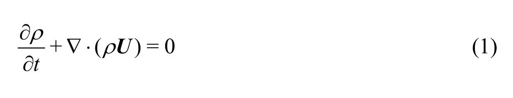
The momentum equation in an absolute frame of reference or in an inertial frame is

where ρ is the density of the fluid,tis the time,U is the absolute velocity of the fluid, f is the body force per unit mass of fluid,pis the pressure,μ is the dynamic viscosity, δ is the identity matrix,▽ represents the Hamilton operator and the superscript T denotes the transpose of a matrix.

Because of the rotating movement of the vehicle,the Coriolis acceleration is involved and the rotating arm tank problem cannot be directly solved in an inertial frame. But if the frame of reference is built on the body of a vehicle, the vehicle will be at rest relatively all the time, thus the standard N-S momentum equation must be modified accordingly due to the difference between an inertial frame and a moving one.

The momentum equation in a body fixed frame of reference is given below, and more details are to be found in Ref. [15].

whereea is the acceleration of the entrainment,ca is the Coriolis acceleration.

Compared with the momentum equation in an inertial frame, the added momentum sources in a body fixed frame of reference is

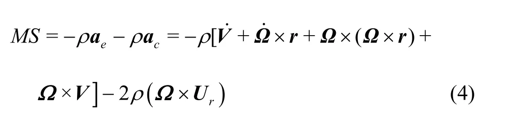
where V and Ω are the linear velocity and the angular velocity of the vehicle, respectively,rU is the relative velocity, r is the relative position vector,and a superscript dot is used to denote the derivative with respect tot.

The multiple reference frames (MRF) method is chosen in the FLUENT, the N-S equation in the MRF can be written as

Compared with the N-S equation in an inertial frame, the added momentum sources can be expressed as

Under the condition of the rotating arm test, the linear velocity of the vehicle =0V , the angular velocityconst =constantΩ

, Eq. (3) becomes the same as Eq. (5). Thus the MRF method is equivalent with the body-fixed frame method.

A semi-relative reference frame method in this paper combines the rotating reference frame and the added momentum source method. The computational domain is separated into two parts, for one part the rotating reference frame is adopted and the other part is in an inertial frame. The center of rotation is the moment center.

The added momentum sources are given below,and the more details are to be found in Ref. [16]

R0is the rotating radius.

Provided that the frame of reference is fixed at an arbitrary point in the vehicle and the absolute velocity of an element of fluid is

In this equation,eUis the velocity of the entrainment.

Since the absolute velocity of an element of fluid is zero far away, the relative velocity at the inlet then is

Under the initial condition, the whole fluid domain is separated into two parts. The domain above the submerging line is called the air field. The volume fraction of the air is set to 1. The pressure above the submerging line is set to 0. The domain under the submerging line is called the water field. The volume fraction of the air is set to 0. The pressure distribution of the water domain under the submerging line is related to the distance to the free surface. The value of the pressure is determined by the functionPd=ρwgδh.wρ is the density of water,gis the acceleration of gravity, andhδ is the distance from any of the water field to the free surface.

2. VOF method

The VOF method is used to simulate the free surface of the vehicle. In order to track the interface between the air and the water, the transport equation of the volume fraction of the water phase is solved[17]

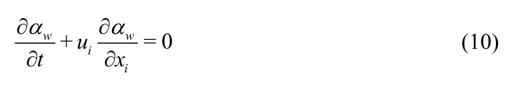
wherewα is the volume fraction of the water. The water volume fraction and the air volume fractionaα satisfy the following equation

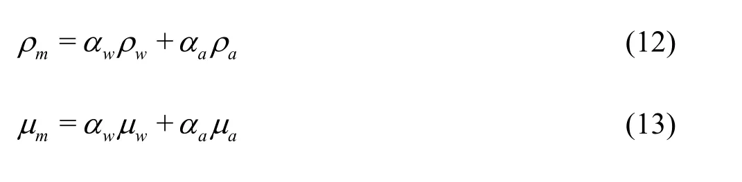
At each control volume, the density and the viscosity of the mixture are calculated by the volume fraction average:

3. Computational model and meshing

The vehicle has a small length width ratio of 1.5.The ratio of the vehicle length to the height is 4. The vehicle is in a symmetric shape. The ratio of the sea gauge to the height of the vehicle is 0.86 under the surface navigation condition, which is treated as a constant in this paper. The side view of the vehicle is shown in Fig. 1. The grid generation includes the surface meshing, the boundary layer meshing, and the volume meshing. The elementary requirements for the surface meshes are the smoothness, the orthogonality,and the uniformity. The most important point is that the surface meshes must exactly capture the characteristics of a given geometry. In order to capture the free surface and the blended wing body vehicle complex shape, a hybrid mesh is adopted as shown in Fig. 1. The meshes near the vehicle are unstructured such as the tetrahedral, the prismatic and the pyramidal.

Fig. 1 (Color online) The computational mesh

To investigate the sensitivity of the results to the grid resolution, three sets of grids are used with 3.0×106, 3.5×106and 4.0×106nodes, respectively (as shown in Fig. 2). The grid densities on the surface vary while the heights of the boundary layer prim cells are fixed among the meshes.

A comparison of the direct resistance of the vehicle is shown in Table 1. The inlet velocities in various cases are 8 Kn, 16 Kn, respectively. It is indicated that the direct resistance of the vehicle reaches a convergent value with the increase of the mesh refinement. The differences between the medium and fine meshes can be accepted. Thus, the medium mesh with about 3.5×106cells is selected as the final grid.

Fig. 2 (Color online) Grid-independent verification for vehicle

Table 1 Comparison of direct resistances of the vehicle

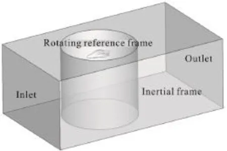
Fig. 3 The computational domain

The computational domain can be a cube or a cylinder, which is separated into two parts, in one part the rotating reference frame (the cylinder part) is adopted, and the vehicle is located in this part, in which the rotating center is the moment center of the vehicle (as shown in Fig. 3). The added momentum source in this part is as shown in Eq. (7). In the other part, an inertial frame is adopted. The velocity condition is applied for the inlet boundary, and the SST -kω turbulent model is adopted to simulate the turbulent flow. The remaining boundaries are set as the zero average static pressure outlet boundaries. It is designated that the water is the first phase while the air is the second phase. The density of the water is 1 025.91 kg/m3,the viscosity coefficient is 0.0012 kg/ m·s. The density of the air is 1.23 kg/m3. The transient calculation is performed by using the explicit VOF method with the geometric reconstruction method to capture the rough shapes of the free surface for about 1 000 steps. Then the steady state calculation is continued with the implicit VOF method until a convergent state is reached. The PISO scheme is adopted in the pressure-velocity coupling method to combine the continuity and momentum equations together and calculate the pressure. The pressure staggering option(PRESTO) is selected for the pressure interpolation,and the second order upwind scheme is used for the vapor volume fraction transport equation.

4. Results and discussions

The dimensional analysis method is used to analyze the results. The resistance of the vehicle consists of three parts: the viscous resistance, the pressure resistance and the wave making resistance.The main parameters are the navigation speedV, the angle of attack α, the drift angle β, the characteristic lengthL, the volume of displacementD,the fluid density ρ, the fluid viscosity μ, the acceleration of gravitygand the radius of gyrationR. The dependent variable is the surface pressure.

Then the related function is expressed as

whereV,L, ρ are chosen as the fundamental quantities. Thus the dimensionless expression is

In this equation, =FrVis the Froude number,which represents the gravity effect.Re=ρVL/μ is the Reynolds number, which represents the viscosity effect. From the dimensional analysis on the resistances in the Ref. [18], it is indicated that both the Froude number and the Reynolds number obtained from modeling experiments should be equal to the corresponding dimensionless quantities in the prototype in small-scale modeling experiments. But we cannot have the sameFrandReat the same time in practice. Compared to the influence of the Froude number, the influence of the Reynolds number on the flow around the vehicles can be ignored when the Reynolds number is larger than 106. The speed of the vehicle in this paper is varied from 4 Kn to 20 Kn.The Reynolds number is about 107. So the influence of the Reynolds number is ignored in this paper.

Thus, when the shape and the operating condition of the vehicle are fixed, the dimensionless parameters can be simplified as

Next, the influence ofFrand /L Ron the vehicle hydrodynamic will be discussed in detail.

5. The influence of Froude number Fr in the direct cruise condition

The influence of the Froude number can be analyzed under the direct cruise condition, in order to neglect the effect of the turning radius. The variation of the pressure resistance coefficient is shown in Fig.4, whereCd-p=Fd-p(1/2ρV2L2) andFd-pis the pressure drag. In Fig. 4, the black line represents the pressure resistance coefficient distribution under the underwater condition, in which the influence of the free surface is neglected. So,dpC-is independent of the Froude number. For the surface navigation, its pressure resistance coefficient against the Froude number (the solid line, as shown in Fig. 4) is in a significant fluctuation distribution. The ratio of the sea gauge to the height of the vehicle is 0.86 under this condition. In fact, the effect of the Froude number onCd-pdepends on the depth of the vehicles below the water surface. The pressure resistance coefficient distribution also varies with the state of submerging.The pressure variation difference between the underwater and surface navigations is mainly due to the wave making resistance, consisting of three parts: the wave resistance at the head of the vehicle, the interference wave resistance of the vehicle body with the head wave, and the scattered wave resistance. The wave making resistance coefficient reaches a valley value when =0.3Frand a peak value when =Fr0.5.

Fig. 4 The pressure resistance coefficient variation against Froude number

The flow characteristics in the cases of these two Froude numbers will be considered. Figure 5 shows the dimensionless wave height distribution of the blended wing body vehicle. An iso-surface is established in the whole domain, and the volume fraction of the air is 0.5. The line located at the central axis of the iso-surface is used to reveal the wave profile. In Fig. 5,Lis the vehicle body length,His the wave height, andxis the position in the flow direction.The lines represent the wave profile distributions for different Froude numbers. As seen from the graph, the interference effects on the position of the stern atFr= 0.3 are quite different from that atFr= 0.5.

Fig. 5 The dimensionless wave height distribution

The contours of the height of the water surface are shown in Fig. 6. The colors represent the heights of the water surface. There are obvious wave troughs in the tail of the vehicle (as pointed by the arrow in Fig. 6). The wave height distribution agrees well with that in Fig. 5 (the circle part).

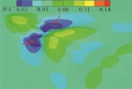
Fig. 6 (Color online) The contours of the height of the water surface at =0.5Fr

Figure 7 is the comparison of the streamline distribution. At =0.3Fr, the wave height distribution is straight at the stern of the vehicle (as shown in Fig.7(a)), because the bow wave troughs counteract the stern wave crest, reducing the wave resistance. And the wave resistance is enhanced at =0.5Fr(as shown in Fig. 7(b)), where both the wave crests overlay each other, inducing a large wave elevation.

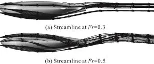
Fig. 7 Comparison of streamline at =0.3Fr , =0.5Fr

The extreme value of wave resistance can also be predicted by thePtheory. The peak point is related to the navigation speed, the vehicle length and the prismatic coefficient. The function can be expressed asmL=f(L,λ,Cp), wheremLis the superposition wave making length, λ is the initial wave length,λ= 2π/gV2,Cpis the prismatic coefficient of the vehicle, andLis the length of the vehicle.

The distance between the first wave crest and the stern wave trough of the vehicle can be expressed asCp L. So the superposition wave making lengthismL=Cp L+ 3/4λ. The wave length can be divided intoninteger waves andqfraction waves,mL=nλ+qλ. Then,Cp L/ λ= (n+q)- 3 /4.P=is introduced to analyze the peak point.Detailed derivation can be found in Ref. [19]. For this blended wing body vehicle, the wave crest is atP= 1.15 (forFr= 0.3) and the wave trough is atP= 2.00 ( forFr= 0.5). The calculated results of the wave resistance peaks agree well with the numerical computation results.

Because of the low length-width ratio, much stronger transverse waves are generated by this kind of vehicles than the general surface ship with a slender body. In addition, the wave length is close to the body length, so there is a strong interference between the bow wave and the stern wave. Thus in summary, the variation range of the resistance against the speedis remarkably larger than that of an average ship, and an appropriate navigation speed is very important for energy saving.

6. The influence of /L R under the turning condition

Figure 8 represents the yaw moment coefficient againstL/Rof the vehicle under the underwater condition, while Fig. 9 represents that under the surface navigation condition.CN=N/(0.5ρV2L3) is the yaw moment coefficient,L/Ris the ratio of the characteristic length of the vehicle to the radius of rotation. Under the underwater condition, the yaw moment coefficient is a linear function of /L R. More details about the maneuvering characteristics of the vehicle under the underwater condition can be found in the Ref. [20]. But under the surface navigation condition, the relationship between the yaw moment coefficient and /L Ris nonlinear. The variation of the yaw moment coefficient is almost linear in the region of small rotating velocity, while the variation becomes small in the region of a large rotating speed.In view of the fact that the yaw moment coefficient is a linear function under the underwater conditions (as shown in Fig. 8), the nonlinear effects may be associated with the shape change of the free surface under various above water conditions.

Fig. 8 The lateral moment rotation derivative under 4 Kn underwater horizontal rotation condition

Fig. 9 The lateral moment rotation derivative under 4 Kn above water horizontal rotation condition

Figure 10 shows the pressure coefficient distributions for different gyration radii under the underwater condition, and Fig. 11 shows the pressure coefficient distributions for different gyration radii under the surface navigation condition. All results are based on the averaged time. The vehicle is located in the Cartesian coordinates. The -Xaxis points to the head of the vehicle, the -Yaxis points to the right wing of the vehicle and the -Zaxis points to the bottom of the vehicle. The origin is at the buoyancy center of the vehicle. The data in Fig. 10, Fig. 11 are derived from the lineX/L= - 0 .375.Cpis the pressure resistance coefficient. The effects of the hydrostatic pressure are excluded both in Fig. 10, Fig. 11.Y/Lis the dimensionless length. It is obvious that with the increase of the rotation radius, the asymmetry of the pressure on left and right sides of the vehicle is gradually decreased. Under the influence of the wall lateral velocity, the pressure increases in the upstream region on the right side, while the pressure decreases in the downstream region on the left side (as shown in Fig.11), which is similar to the tendency of the pressure distribution under the above water condition. It is indicated that the influences of the rotating speed on the wall dynamic pressure are mainly the same under the underwater and above water conditions.

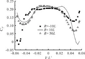
Fig. 10 The lateral moment rotation derivative under 4 Kn underwater horizontal rotation condition

However, the rotating speed can also affect the free surface patterns. The free surface distributions of the wave against the radius under the vehicle are as shown in Fig. 12. It is shown that the free surface patterns are similar under the conditions of a small rotating speed and a large rotating radius (as shown in the middle and right views in Fig. 12). Therefore, the feedback yaw moment variation is mainly caused by the dynamic pressure distributions, varying linearly under a small rotating velocity condition. Moreover,under the conditions of a large rotating speed and a small rotating radius (as shown in the left view in Fig.12), the free surface shape changes remarkably, and the water depth in the downstream region on the left side increases significantly. Consequently, the hydrostatic pressure is increased in the downstream region,therefore, the increase of the overall yaw moment slows down when the rotating speed becomes larger(as the nonlinear trend shown in Fig. 9).

Fig. 12 (Color online) The free surface patterns for the vehicle with different radii

7. Conclusions

The wave characteristics of the blended wing body vehicle with a small length-width ratio, a deep draft and a high speed are investigated in the present paper, to provide some reference for the similar type of vehicles.

(1) Based on the VOF implicit method, the wave resistance characteristics of the blended wing body vehicle are obtained. The wave making resistance is consistent with the result obtained by thePtheory.

(2) The wave length is equal to the body length,and the wave interference effects are significant. The wave making resistance coefficient against the speed sees a remarkable fluctuation, so an economic navigation speed should be chosen carefully.

(3) The horizontal rotation maneuvering characteristics are nonlinear and more complex than under the underwater condition, which is caused by the unsymmetrical wave pattern under the vehicle.

A prototype of the blend wing body vehicle is in production. The results of the hydrodynamic force can be obtained from the lake experiment, which will be discussed in the following work.

[1] Dehpanah P., Nejat A. The aerodynamic design evaluation of a blended-wing-body configuration [J].Aerospace Science and Technology, 2015, 43: 96-110.

[2] Liebeck R. H. Design of the blended wing body subsonic transport [J].Journal of Aircraft, 2012, 41(1): 10-25.

[3] Rahman N. U., Whidborne J. F. Propulsion and flight controls integration for a blended-wing-body transport aircraft [J].Journal of Aircraft, 2009, 47(2): 895-903.

[4] Lyu Z., Martins J. Aerodynamic design optimization studies of a blended-wing-body aircraft [J].Journal of Aircraft, 2014, 51(5): 1604-1617.

[5] Qin N., Vavalleb A., Moigne A. L. et al. Aerodynamic considerations of blended wing body aircraft [J].Progress in Aerospace Sciences, 2004, 40(6): 321-343.

[6] Wu Z., Cao Y. Numerical simulation of airfoil aerodynamic performance under the coupling effects of heavy rain and ice accretion [J].Advances in Mechanical Engineering, 2016, 8(10): 1-9.

[7] Su W., Cesnik C. E. S. Nonlinear aeroelasticity of a very flexible blended-wing-body aircraft [J].Journal of Aircraft, 2010, 47(5): 1539-1553.

[8] Brower T. P. L. Design of a manta ray inspired underwater propulsive mechanism for long range, low power operation [D]. Doctoral Thesis, Boston, USA: Tufts University,2006.

[9] Stevens G. M. W. Conservation and population ecology of manta rays in the Maldives [D]. Doctoral Thesis,Yorkshire, UK: University of York, 2016.

[10] Dewar H. D., Mous P., Domeier M. et al. Movements and site fidelity of the giant manta ray, Manta birostris, in the Komodo Marine Park, Indonesia [J].Marine Biology,2008, 155(2): 121-133.

[11] Zhou C. L., Low K. H. Better endurance and load capacity:An improved design of manta ray robot (RoMan-II) [J].Journal of Bionic Engineering, 2010,7(4): S137-S144.

[12] Chen X., Liang H. Wavy properties and analytical modeling of free-surface flows in the development of the multi-domain method [J].Journal of Hydrodynamics,2016, 28(6): 971-976.

[13] Yang X. Y., Zhang H. H., Li H. T. Wave radiation and diffraction by a floating rectangular structure with an opening at its bottom in oblique seas [J].Journal of Hydrodynamics,2017, 29(6): 1054-1066.

[14] Raven H. C. Numerical and hybrid prediction methods for ship resistance and propulsion [M]. New York, USA: John Wiley and Sons, 2017.

[15] Hu Z., Lin Y. Computing the hydrodynamic coefficients of underwater vehicles based on added momentum sources[C].The 18th International Offshore and Polar Engineering Conference, Vancouver, BC, Canada, 2008.

[16] Wu X., Hung C., Yang L. et al. A semi-relative reference frame method for manoeuvring simulation in hydrodynamics [C].The 14th Asia Congress of Fluid Mechanics,Hanoi and Halong, Vietnam, 2013.

[17] Passandideh F. M., Roohi E. Transient simulations of cavitating flows using a modified volume-of-fluid (VOF)technique [J].International Journal of Computational Fluid Dynamics, 2008, 22(1-2): 97-114.

[18] Tan Q. M. Dimensional analysis with case studies in mechanics [M]. Berlin, Heidelberg, Germany: Springer,2011, 27-29.

[19] Sheng Z. B., Liu Y. Z. Theory of ship (volumes first) [M].Shanghai, China: Shanghai Jiao Tong University Press,2004(in Chinese).

[20] Wu X. C., Wang Y. W., Huang C. G. et al. Study on maneuvering characteristics of blended wing body vehicle[J].Scientia Sinica Technologica, 2015, 45(4): 415-422(in Chinese).