Jianghao LI and Li DONG

1Key Laboratory of Earth System Modeling and Prediction, China Meteorological Administration, Beijing 100081, China

2State key Laboratory of Numerical Modeling for Atmospheric Sciences and Geophysical Fluid Dynamics (LASG),Institute of Atmospheric Physics (IAP), Chinese Academy of Sciences, Beijing 100029, China

3State Key Laboratory of Severe Weather (LaSW), Chinese Academy of Meteorological Sciences,China Meteorological Administration, Beijing 100081, China

4College of Earth and Planetary Sciences, University of Chinese Academy of Sciences, Beijing 100049, China

ABSTRACT If an explicit time scheme is used in a numerical model,the size of the integration time step is typically limited by the spatial resolution.This study develops a regular latitude–longitude grid-based global three-dimensional tracer transport model that is computationally stable at large time-step sizes.The tracer model employs a finite-volume flux-form semi-Lagrangian transport scheme in the horizontal and an adaptively implicit algorithm in the vertical.The horizontal and vertical solvers are coupled via a straightforward operator-splitting technique.Both the finite-volume scheme’s onedimensional slope-limiter and the adaptively implicit vertical solver’s first-order upwind scheme enforce monotonicity.The tracer model permits a large time-step size and is inherently conservative and monotonic.Idealized advection test cases demonstrate that the three-dimensional transport model performs very well in terms of accuracy,stability,and efficiency.It is possible to use this robust transport model in a global atmospheric dynamical core.

Key words: tracer transport,numerical stability,latitude–longitude grid

1.Introduction

To improve the forecast or simulation skill,global weather and climate models generally resolve more atmospheric motions by increasing their spatial resolutions,such as in global storm-resolving or cloud-resolving models (e.g.,Satoh et al.,2019;Stevens et al.,2019).Moreover,most weather and climate models use higher resolutions in the vertical than in the horizontal.As the horizontal and vertical spatial resolution increases,the advective Courant number (or Courant–Friedrichs–Lewy,CFL) becomes the primary factor that constrains the model time-step if an explicit time scheme is applied.The Courant number should be less than a specific scheme-dependent constant (typically,unity);otherwise,the model would be numerically unstable.This Courant number limitation is even stricter for global models with a latitude–longitude grid because of the convergence of the meridians at the poles (Lin and Rood,1996;Weller et al.,2023).

For atmospheric models that use the latitude–longitude grid,there are a few alleviations to the Courant number limitation.Semi-Lagrangian time-stepping techniques,which are widely used in atmospheric models,allow for larger timestep sizes than the CFL-constrained Eulerian methods do(Wood et al.,2014);however,the classical semi-Lagrangian transport scheme does not formally conserve the total mass(Staniforth and Côté,1991;Diamantakis,2014).The lack of mass conservation for certain quantities is inadequate for long-term simulations and for the overall accuracy of atmospheric models.

Another approach to removing the Courant number restriction is using implicit advection schemes.The virtue of implicit methods is the attractive unconditional stability properties,thus allowing large Courant numbers in terms of stability (Hundsdorfer and Verwer,2003).However,one disadvantage of implicit time-stepping methods is the computational cost of solving a matrix equation.Other disadvantages of implicit advection schemes include large phase errors when using large time-step sizes and difficulties in achieving monotonicity (Chen et al.,2017).

An alternative straightforward approach to alleviating the CFL constraint on a latitude–longitude grid is the application of a quasi-uniform spherical grid (Williamson,2007;Staniforth and Thuburn,2012).For instance,the pole problem on a latitude–longitude grid is almost completely avoided by using a cubed-sphere or icosahedral grid.A quasi-uniform spherical grid,however,lacks the latitudinal regularity of the rotational Earth.Additionally,the internal boundary or singularity of the polygon needs to be specifically addressed,which could lead to computational mode and grid imprinting(Weller,2012).

There are also several desired properties of numerical schemes for tracer transport,such as monotonicity,shape preservation,positivity,and mass conservation [refer to Lauritzen et al.(2011) for a comprehensive review].Flux-corrected transport (FCT) is a monotonicity-preserving method that computes and limits flux using both a low-order monotonic method and a higher-order scheme (e.g.,Zalesak,1979;Book et al.,1981;Boris and Book,1997).The slopelimiter method (LeVeque,2002;Durran,2010) is another approach that estimates the flux at the cell interface by fitting a piecewise parabola to a finite-volume average of the transported scalar field.These parabolas are subsequently modified to ensure monotonicity is preserved.This study uses both methods to obtain monotonicity.

We have developed a new shallow-water model of the Grid-point Atmospheric Model of IAP (Institute of Atmospheric Physics) LASG (State key Laboratory of Numerical Modeling for Atmospheric Sciences and Geophysical Fluid Dynamics) (Li et al.,2020),and a baroclinic dynamical core on the latitude–longitude grid is also being developed.The tracer transport module is a crucial component of any weather or climate model.This study takes a further step towards creating a full model by designing a global atmospheric tracer transport model on a regular latitude–longitude grid.First,the FFSL tracer transport algorithm developed by Lin and Rood (1996) is employed horizontally.The semi-Lagrangian property of the FFSL guarantees computational stability when the zonal Courant number is greater than unity,reducing the restrictive limitations on the polar regions.Second,an adaptively implicit vertical transport scheme (Shchepetkin,2015;Wicker and Skamarock,2020;Li and Zhang,2022) is adopted to alleviate the vertical stability limitations.The time-step size in the tracer model will be significantly improved by combining these two approaches.This study presents the computational scheme of the threedimensional transport model,along with the accuracy,stability,and monotonicity of the model.

The remainder of this manuscript is organized as follows.Section 2 describes the horizontal and vertical transport solvers in detail.Section 3 presents results from several well-known idealized two-dimensional and three-dimensional test cases,and a brief conclusion is provided in section 4.

2.Horizontal and vertical solvers

We define the horizontal and vertical grid structures used in this study before introducing the solvers in detail.A regular latitude–longitude grid is used in the horizontal discretization,where winds and tracers are staggered with the Arakawa C-grid (Arakawa and Lamb,1977).The wind component is defined at the middle of the cell interface,while the tracer concentration is defined at the cell center and the Earth’s poles.We use a stationary,non-uniform,massbased,and terrain-following vertical coordinate (Kasahara,1974;Simmons and Burridge,1981;Laprise,1992),with the positive direction pointing downward,and top-down numbering.A Lorenz-type staggering is adopted in the vertical,which means that the vertical coordinate velocity and vertical mass flux are defined at half levels,and the tracer mass-mixing ratio is defined at full levels.

With a general vertical coordinate η,the tracer conservation equation without sources or sinks can be written as

where π is the hydrostatic pressure (Laprise,1992),∂π/∂η is the pseudo-density,andqis the tracer mixing ratio.∇η·()represents the horizontal divergence operator,which can be discretized based on the Gauss theorem.Vhis the two-dimensional horizontal velocity vector,and η˙ is the vertical coordinate velocity.For the purpose of spatial discretization,the layer-averaged formulation [Eq.(12) in Zhang et al.(2020)] is used in this study.Vhandqrepresent layer-averaged states;consequently,the tracer equation can be further expressed as

where δπ denotes the layer mass in a full level (k),δπk=πk+1/2-πk-1/2.The δ operator in the third term denotes the difference between two half levels,which is defined at the full levels:

To implement the adaptively implicit vertical transport scheme,the mass-weighted vertical velocityis split into explicit and implicit velocities for the explicit and implicit transport parts,respectively.Thus,the equation can be semi-discretized as

where the explicit and implicit vertical velocities are partitioned from the full vertical velocity:

where the splitting parameter β is a transition function responsible for the splitting of the vertical velocity between a fully explicit solver (β=1) and a fully implicit solver(β=0),which is determined by the local Courant number.We do not describe the calculating formulation of β and related parameters since these can be found in Wicker and Skamarock (2020).This approach has the advantage of rendering vertical advection stable and maintaining high accuracy in locations with low Courant numbers.

The fractional step,also known as operator-splitting,is attractive for solving the three-dimensional equation because of its efficiency and high accuracy in each spatial dimension (e.g.,Lin and Rood,1996,1997;LeVeque,2002;Putman and Lin,2007).The operator-splitting is applied between horizontal and vertical operators to make it simpler to implement an implicit integration scheme in the vertical,although the operator-splitting is first-order accurate in time.A form of Strang splitting (Strang,1968) can also be used to achieve second-order accuracy.After calculating the horizontal operator,the updated tracer mass-mixing ratio is used for the vertical operator.

The computational procedures are as follows:

(i) Calculate the horizontal flux for the intermediate variable using

where the superscriptsnand * denote the state at time levelnand intermediate time level,respectively.In our model,the Lin and Rood (1996) FFSL approach is used,which is based on forward Euler explicit time differencing (a two time-level scheme).The essence of the FFSL method is that the two-dimensional flux divergence is split into two orthogonal one-dimensional flux-form transport operators.The flux is approximately equal to the air-mass flux times the tracer mixing ratio on the cell interface in a one-dimensional direction.Either the piecewise linear van Leer method or the Piecewise Parabolic Method (PPM,Colella and Woodward,1984;Carpenter et al.,1990) can be used to reconstruct the tracer in a mesh cell by using mean values of surrounding cells.We choose the PPM for our model because of its accuracy and computational efficiency.In addition,a monotonicity constraint (or slope-limiter) can be imposed on the onedimensional discrete solution,but,due to dimensional splitting,this does not ensure exact monotonicity in the overall two-dimensional solution (Lin and Rood,1996;Kent et al.,2012).The slope-limiter would damp the numerical oscillations but introduce diffusion in the numerical solutions.We used the modified version of the PPM limiter from Appendix B of Lin (2004) for both the horizontal and vertical advections.A minor correction regarding the limiter is noted in the appendix of this paper.

A semi-Lagrangian approach is also used in the longitudinal (east–west) direction on the latitude–longitude grid to alleviate the pole problem.The flux across cell interfaces is calculated by integrating the swept volume over a large number of upstream zonal cells.This approach enlarges the upwindbiased computation stencil that relaxes the CFL linear stability constraint,especially near the poles,as stated in section 3 of Lin and Rood (1996).Since the method is in the fluxform (the FF abbreviation in FFSL),it guarantees the total tracer mass conservation,whereas the conventional method that tracks computational grid points does not make this guarantee.The pure Eulerian counterpart is used in the meridional(north–south) direction,so the time-step size is only constrained by the meridional Courant number.

For comparison,we also implement a third-order upwind flux formulation combined with a third-order Runge–Kutta (RK3) time integrator (Wicker and Skamarock,2002;hereafter RK3O3) in the horizontal solver.Unlike FFSL,RK3O3 is a method of lines (Hyman,1979;Shchepetkin,2015),where the spatial and temporal discretizations are decoupled and treated separately.The FCT algorithm (Zalesak,1979) is applied in RK3O3 to restore positive definiteness or monotonicity.It should be noted that the FCT operator can be applied either on each sub-step or the last sub-step of the RK3 scheme.In our tests,the former guarantees strict monotonicity,while the latter cannot (see section 3.1).

(ii) Update the mass-weighted mixing ratio in the vertical explicit residual with

whereq∗=(δπq)∗/δπn+1,the superscript ** denotes the state at intermediate time level,and the layer massδπn+1can be obtained by the continuity equation in the dynamical core of a full model.The layer mass is unchanged with time in the passive tracer advection tests.The explicit vertical velocityis used in the one-dimensional finite-volume scheme.As in the horizontal solver,we can obtain the vertical flux at half levels by using the third-order upwind flux operator or the PPM finite-volume method.The third-order upwind flux operator combines with the RK3 time-integrator method (RK3O3),whereas the PPM flux operator is equipped with the forward Eulerian time integration.Similarly,the FCT and slope-limiter can be imposed on the RK3O3 and PPM flux operators,respectively.The performance of these schemes will be evaluated by the following test cases.

(iii) At the last step,update the tracer using an implicit algorithm with

Because it is the only inherently monotonic linear scheme (Godunov and Bohachevsky,1959),the first-order upwind scheme is chosen to calculate the vertical mass flux at the half interface.While other higher-order nonlinear schemes are theoretically possible,the first-order upwind method is typically more cost-effective.Then,the mixing ratio at a new time level can be obtained byqn+1=(δπq)n+1/δπn+1.Since each unknowndepends on its upperneighbors (subscriptkis used for the variable located in the full layer in the vertical direction),the above set of equations form a tridiagonal system in a vertical column.The system of linear equations can be solved with a tridiagonal matrix algorithm.

The summary of flux operators and monotonic limiters used in the model for the idealized tests is provided in Table 1.

Table 1.List of the horizontal and vertical flux operators,along with the corresponding limiters in the tracer transport model.

3.Transport tests

This section discusses the results of the transport model runs using four standard passive-tracer transport test cases.The test cases have varying degrees of complexity in two and three dimensions.All the test cases use a prescribed time-(in)dependent flow field.The accuracy and properties of the two-dimensional transport scheme are evaluated using two-dimensional horizontal tests.Two additional three-dimensional passive-tracer transport test cases from Kent et al.(2014) are performed in our model.They are used to demonstrate the accuracy of horizontal–vertical coupling and the viability of the adaptively implicit vertical transport algorithm.

Error norms can be calculated because the final tracer distribution for each test is ideally equal to the initial condition or is given analytically.The error norms of ℓ1,ℓ2,ℓ∞are defined as in Williamson et al.(1992):

where H denotes the computational solution,HTdenotes the analytic or reference solution,m ax∀ selects the maximum value from a given field,andIis the global two-dimensional integral,

or the global three-dimensional integral,

3.1.Two-dimensional solid-body rotation test

The test case of solid-body rotation over the sphere(Williamson et al.,1992;test case 1) is widely used to assess two-dimensional advection schemes.The nondivergent zonal and meridional velocities are given by:

where λ and φ are longitude and latitude,respectively.The maximum wind speedu0=2πa/12 days ≈38.61 m s-1andais the radius of the Earth.α denotes the flow orientation angle to the equator,with α=90º corresponding to the advection of the solid body crossing the pole.Ideally,the solid body translates without changing shape and returns to its initial position after one rotation (12 days).We evaluate the horizontal advection solver from different aspects using three initial distributions.

First,to evaluate the positive definitiveness or monotonicity of the advection algorithm with limiters,the initial shape is set as two-slotted cylinders.The two-slotted cylinders centered on (λ0,ϕ0)=(3π/2,0) are defined as

where (λ1,φ1)=(λ0-π/6,φ0),(λ2,φ2)=(λ0+π/6,φ0),r0=a/2,andr1andr2are the great circle distances,

from (λ1,φ1) and (λ2,φ2),respectively.

Figures 1 and 2 show the results of this test case using the RK3O3 and FFSL schemes with and without the monotonic limiters.The spatial resolutions are 2º,1º,and 0.5º,and,when α=90◦,the maximum time-step sizes of the RK3O3 scheme are 288 s,72 s,and 18 s.This guarantees that the Courant number is approximately constant (～1.43)at the three resolutions.The same time-step sizes as RK3O3 are applied to FFSL for comparison,although FFSL can take larger time-step sizes.Both schemes cannot prevent nonphysical under-and overshoots in the absence of limiters,as evidenced by the values less than 0.1 or greater than 1.Since RK3O3 itself possesses some degree of dissipation(Wicker and Skamarock,2002;Skamarock and Gassmann,2011),the under-and overshoots are slightly smaller in magnitude than the results of the FFSL scheme.The monotonic limiter would effectively eliminate the undershoots and overshoots,as shown in Fig.2.In our model,it should be noted that the FCT flux limiter was activated during each RK3 time-integrator sub-step.If the FCT limiter is only applied on the last RK3 sub-step,undershoots and overshoots will still exist (not shown).

Next,we evaluate the model simulating a solid body passing over the pole.The initial cosine-bell tracer distribution is

where the radiusR=a/3 and the maximumh0=1000;rdenotes the great circle distance between a position(λ,φ)and the center of the cosine bell (λc,φc)=(3π/2,0).

Figure 3 presents the transport of the cosine-bell structure over the North Pole using the RK3O3 and FFSL schemes with their respective FCT flux-and slope-limiters.The spatial resolution is 1º.First,set the time-step size to 72 s,which corresponds to the longitudinal and meridional Courant numbers of～1.43 and～0.025,respectively.When using much larger time-step sizes,the model with the RK3O3 scheme tends to become unstable.In other words,the RK3O3 permits a maximum Courant number of approximately 1.43 for stability.As shown in Figs.3a and b,neither scheme exhibits significant distortions.Using the FFSL scheme,the shape of the cosine bell undergoes stretching in the flow direction,which is typically observed in monotonic finite-volume advection algorithms (e.g.,Lin and Rood,1996;Nair and Machenhauer,2002;Jablonowski et al.,2006).

In practice,the FFSL scheme allows for much longer time-step sizes.We increase the time-step size to 1440 s so that the zonal and meridional Courant numbers are～28.64 and～0.5,respectively,as shown in Fig.3c.When passing over the North Pole,the cosine bell deforms slightly;if larger time-step sizes were used,the deformation would be more pronounced.However,no deformation was observed when the rotation angle was 0◦or 45º (not shown).Therefore,the deformation possibly results from the large curvature of the Earth near the pole.Within the FFSL scheme,the departure point is only calculated in the zonal direction.In general,the larger the time-step size,the larger the halo width for parallel distributed-memory communication,which has an additional negative effect on the computational efficiency.Specialized parallel optimization could be conducted to mitigate this overhead,such as limiting the large halo within the polar region and using asynchronous communication,but it is beyond the scope of this work.Nevertheless,it is still worth pointing out that the FFSL scheme permits a much larger time-step size than the RK3O3 scheme does.

To further evaluate the accuracy of the two advection schemes,the advection of a Gaussian hill was carried out.The Gaussian hill (Nair and Lauritzen,2010) is defined as

whereb0=5 defines the width of the Gaussian hill.(X,Y,Z)are the three-dimensional absolute Cartesian coordinates corresponding to the spherical (λ,φ) coordinates:

The center of the Gaussian hill (Xc,Yc,Zc) is calculated by substituting (3π/2,0) for (λ,φ) in Eq.(20).This tracer distribution function is continuously differentiable,so the theoretical accuracy order of the horizontal solver can be estimated from the convergence rate of the error norms (e.g.,Nair and Lauritzen,2010;Skamarock and Gassmann,2011;Kent et al.,2012).

Unlike in Kent et al.(2012),where the spatial resolution is variable and the time-step size is constant,in this case we continuously change the time-step size to hold the maximum zonal Courant number fixed.For α=0◦,the solid body is advected around the equator.The spatial resolutions range from 2º to 0.5º,and the corresponding time-step sizes are 2880 s,1440 s,and 720 s.A constant Courant number of～0.5 results from this configuration.For α=45◦,the timestep sizes are 480 s,120 s,and 30 s,which result in a maximum Courant number of～1.7.For α=90◦,the Gaussian bell is advected across the poles with time-step sizes of 288 s,72 s,and 18 s,which give a constant Courant number of～1.43.

The convergence plots for ℓ2and ℓ∞for the unlimited and limited variations of the RK3O3 and FFSL schemes under three rotation angles are shown in Fig.4.When the axis of the solid-body rotation coincides with the polar axis(α=0◦),the convergence rate is strictly at the theoretical third-order for both the RK3O3 and FFSL schemes without limiters.Additionally,the FFSL’s absolute errors are about an order of magnitude smaller than those of RK3O3.In the case of two-dimensional advection,the convergence rates are usually below third-order.Furthermore,the absolute errors generated by the two schemes do not significantly differ in their two-dimensional motion.Note that limiters typically reduce the third-order convergence to second-order convergence and increase the absolute errors,especially for the FFSL scheme.Overall,the limiter-based variations of these two schemes allow for approximately second-order convergence rates.

3.2.Two-dimensional moving vortices

This test combines the previous solid rotation flow with a deformational (nondivergent) vortex flow.Although the deformational flow field varies in time and space,analytical solutions are readily available.The deformational flow creates two vortices on the polar opposite sides of a rotating sphere.The vortices are transported at an angle α to the east of the equator in a background solid-body rotation.Here,the rotation angle is 90º,which corresponds to the crosspolar flow.Other parameters for this test case follow Nair and Jablonowski (2008) and Norman and Nair (2018).The initial positions of the two vortices are (3π/2,0) and(π/2,0).It takes 12 days for the two vortices to complete one rotation over the poles.

Figures 5a and c present the numerical solution after 12 days of simulating the tracer field using the RK3O3 and FFSL schemes.To guarantee monotonicity,both the FCT flux limiter and slope-limiter are used.There is no significant difference between the two results.Figures 5b and d give plots of the final solution and the exact solution along the equator,showing that the two schemes yield nearly identical solutions and diffusions due to the use of limiters.The phase error of FFSL is slightly smaller than that of RK3O3.

The convergence rates for this test case are shown in Fig.6a.The two schemes’ convergence rates are less than second order from 2º to 1º and approximately second order from 1º to 0.5º.The difference in the absolute errors between the two schemes is negligible.The present performance agrees with the previous simulations.However,the advantage of the FFSL scheme over the RK3O3 scheme is that it allows for a much larger time-step size.The sensitivity of the FFSL to the time-step size is displayed in Fig.6b.We conduct experiments with time-step sizes of 20 s,40 s,80 s,and 160 s and a fixed horizontal resolution of 0.5º.A larger time-step size does not significantly affect the error norms,which is another advantageous feature of FFSL.

3.3.Three-dimensional deformational flow

The test cases presented in the previous two subsections demonstrate the FFSL’s accuracy and its capacity for increasing the time-step size horizontally by contrasting it with the results of RK3O3.The vertical advection scheme,however,also influences the overall accuracy and stability of the real three-dimensional advection process.Furthermore,atmospheric tracers are often observed to have functional relationships in the real world;thus,transport schemes,such as those used in chemistry models,should not disrupt those functional relationships.

Here,we assess the advection scheme’s ability to maintain the functional relationships using the three-dimensional deformational flow test [test 1-1,described in Kent et al.(2014)].The prescribed wind velocities and tracer mixing ratios are described in Kent et al.(2014) and Hall et al.(2016).The three-dimensional winds stretch the tracers (the nonlinearly correlatedq1andq2,both of which have spherical initial shapes,andq3,which has an initial shape of two-slotted ellipses) over the first six days.When the tracers return to their original shapes and positions after being reversed by the flow,it is possible to calculate the error norms.On day 6,the tracer field has the most deformation.

The horizontal spatial resolution is 1º,with 60 uniformly spaced vertical levels in the height coordinate,as recommended in the Dynamical Core Model Intercomparison Project (DCMIP) test document.Specifically,we use a timestep size of 600 s and maximum Courant numbers of approximately 0.44,0.17,and 0.02 in the longitudinal,meridional,and vertical directions,respectively.The adaptively implicit vertical advection algorithm is not activated because the wind speed is much weaker in the vertical direction (small Courant number).As a result,the simulation results of the adaptively implicit algorithm are the same as those of the fully explicit algorithm,which is expected and verified in this test.

We first assess the performance of different flux operators used by the horizontal and vertical solvers in the threedimensional transport model.On day 6,when the tracers stretch to their maximum,Fig.7 presents the horizontal cross-sections of the tracerq3fields at a height of 4.9 km via four combinations of two horizontal flux operators and two vertical flux operators.Figure 8 gives the results on day 12 when the tracers return to their initial positions.In addition,to enforce the monotonicity of the advection process,the slope-limiter and FCT limiter are applied to the advection algorithms.In this way,the tracer distributions reflect the numerical properties of the advection algorithms.

The FFSL horizontal solver in combination with either the vertical PPM or RK3O3 algorithm allows monotonicity and generates nearly identical simulations,as shown in Figs.7a and b and Figs.8a and b.The overall shape and features of the tracer distribution are well preserved.The horizontal RK3O3 solver in combination with either the vertical PPM or RK3O3 algorithm causes some undershoots in the simulations.The undershoots are very small (0.099 and 0.098,the analytical value is 0.1),as shown in Figs.7c and d and Figs.8c and d.When comparing the maximum values of the four combinations,the slope-limiter with the FFSL has greater dissipation than the FCT limiter with RK3O3 does for the horizontal solver.The FCT limiter with RK3O3 has a larger degree of dissipation than the slope-limiter with PPM does for the vertical solver.However,these differences are not significant.If computational efficiency is a concern,a combination of the horizontal FFSL and vertical PPM is preferable.

In addition,this test can objectively evaluate the tracer model’s ability to preserve the correlations between two tracer fields.The first tracer field (q1) is specified as two cosine bells.The second tracer field (q2) is nonlinearly correlated with the first tracer (q2=0.9-0.8).We calculate the real mixing (ℓr),range-preserving unmixing (ℓu),and overshooting (ℓo) forq1andq2,as described in Lauritzen and Thuburn (2012) and Kent et al.(2014).

The correlation plots and the mixing diagnostics,as shown in Fig.9,demonstrate that there is no overshooting for the combination of the horizontal FFSL with the vertical PPM (ℓo=0.0).The other three configurations,however,exhibit slight overshoots.Moreover,this combination yields the smallest real mixing and unmixing values.The scatter plots also demonstrate that this combination best preserves the correlations.

3.4.Three-dimensional Hadley-like meridional circulation

The final experiment is Test Case 1 of the Kent et al.(2014) test suite.The deformational flow mimics the Hadley-like meridional circulation as prescribed in the experiment.The initial tracer field is a quasi-smooth cosine profile.Halfway through the simulation,the designed flow is reversed,and the tracers return to their initial shapes and positions,which provides an analytical solution at the end of the run.We can investigate the effect of the horizontal–verticalsplitting method on the accuracy of the scheme.Here,we first demonstrate that the adaptively implicit vertical advection algorithm can increase the time-step size in this case.The numerical convergence rates of several combinations of horizontal and vertical flux operators are then assessed.

Based on the analysis in the preceding subsection,the FFSL scheme and the PPM-based flux operator are used in the horizontal solver and the explicit part of the vertical solver,respectively.We keep the horizontal and vertical resolution constant while increasing the time-step size.The horizontal resolution is 1º with 180 vertical levels (1◦L180).The time-step sizes are 120 s,240 s,360 s,and 450 s,respectively corresponding to maximum vertical Courant numbers of 0.59,1.18,1.76,and 2.21.

The vertical–meridional slices of the tracer field along the 180 longitude line att=12 hours andt=24 hours are shown in Fig.10 and Fig.11 using the fully explicit and adaptively implicit schemes,respectively.The results of the fully implicit algorithm are also shown for reference.Att=12 hours,the tracer field deforms to its maximum extent.Att=24hours,the tracer field closely resembles its initial phase,although there are some deviations or gaps near 30◦N/S,where the tracer field experiences the greatest stretch.The simulation results of the adaptively implicit and fully explicit algorithms are nearly identical,as expected,when the vertical Courant number falls within the stability limitation (i.e.,0.59 and 1.18).The diffusive property of the fully implicit algorithm is apparent,especially for the gapping at approximately 30ºN/ºS.This is reasonable because the first-order upwind algorithm within the implicit scheme produces the diffusion.In the simulations using the fully explicit algorithm,as the vertical Courant number increases,some abnormal values arose and even caused the model to crash.However,neither the adaptively implicit nor fully implicit scheme produces any abnormal values,and the model remained stable with these two schemes.The former has much less diffusion than the latter at the same time levels.In other words,the adaptively implicit scheme diffuses selectively,whereas the fully implicit scheme yields diffusion almost everywhere.As a result,the adaptively implicit scheme can be implemented well in practical applications.

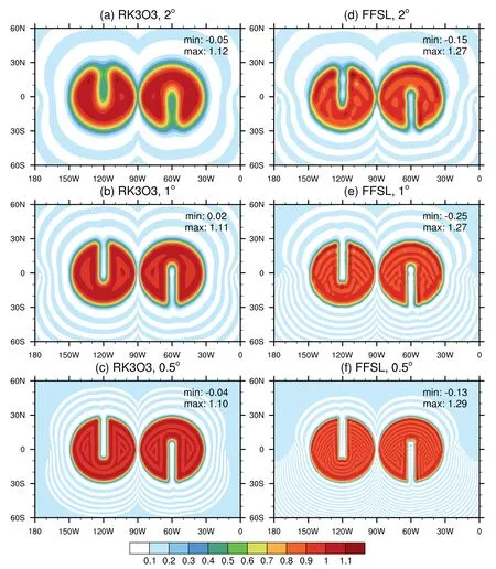
Fig.1.Solid-body rotation of two-slotted cylinders with α=90◦ for spatial resolutions of 2◦ (upper row),1◦ (center row),and 0.5◦ (lower row) using RK3O3 (left column) and FFSL (right column) schemes without limiters at day 12.The minimum (min) and maximum (max) of the simulations are shown in each panel.

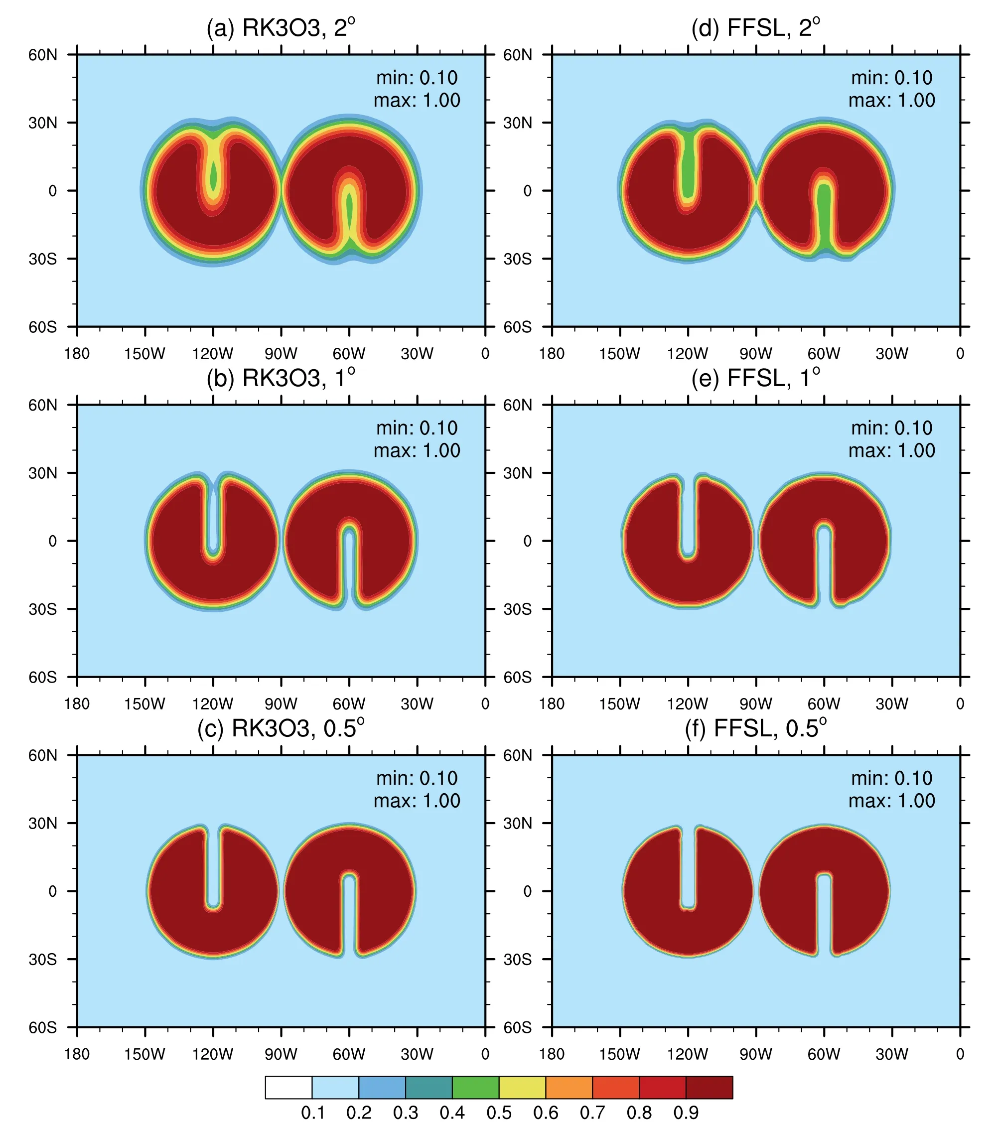
Fig.2.As in Fig.1 but the FCT limiter is applied at each sub-step of the RK3 time integrator,and the monotonic slopelimiter is used for the FFSL scheme.

Fig.3.Snapshots of the cosine bell passing over the North Pole (the outer circle is located at 30◦N) at a resolution of 1◦ with the(a) RK3O3 and (b,c) FFSL schemes.The contour intervals are 100 m,and the zero contour is omitted.The time-step sizes used in the test are also shown in the title of each panel.

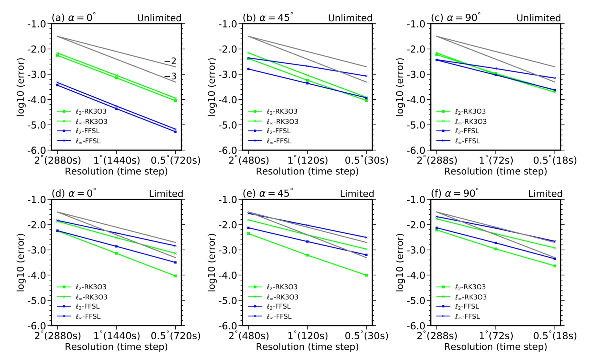
Fig.4.Numerical convergence rates of ℓ2 and ℓ∞ for the unlimited (upper row) and limited (bottom row) variations of the RK3O3 and FFSL schemes in the Gaussian hill rotation test case for different rotational angles (α=0◦,45◦,90◦).The second-and third-order convergence rates (top and bottom,respectively) are plotted as gray lines on each plot.

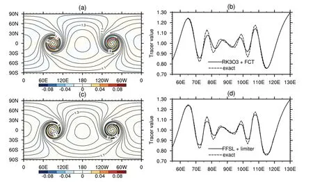
Fig.5.Contour plots (a,c) of the moving vortices at day 12 computed with the limited variations of (a,b) RK3O3 and (c,d)FFSL.The contours in (a,c) are the computational solutions,and the shaded color indicates the difference between the computational and analytical solutions.Panels (b) and (d) show the final solutions along the equator.The spatial resolution is 1º,and the time-step size is 90 s.

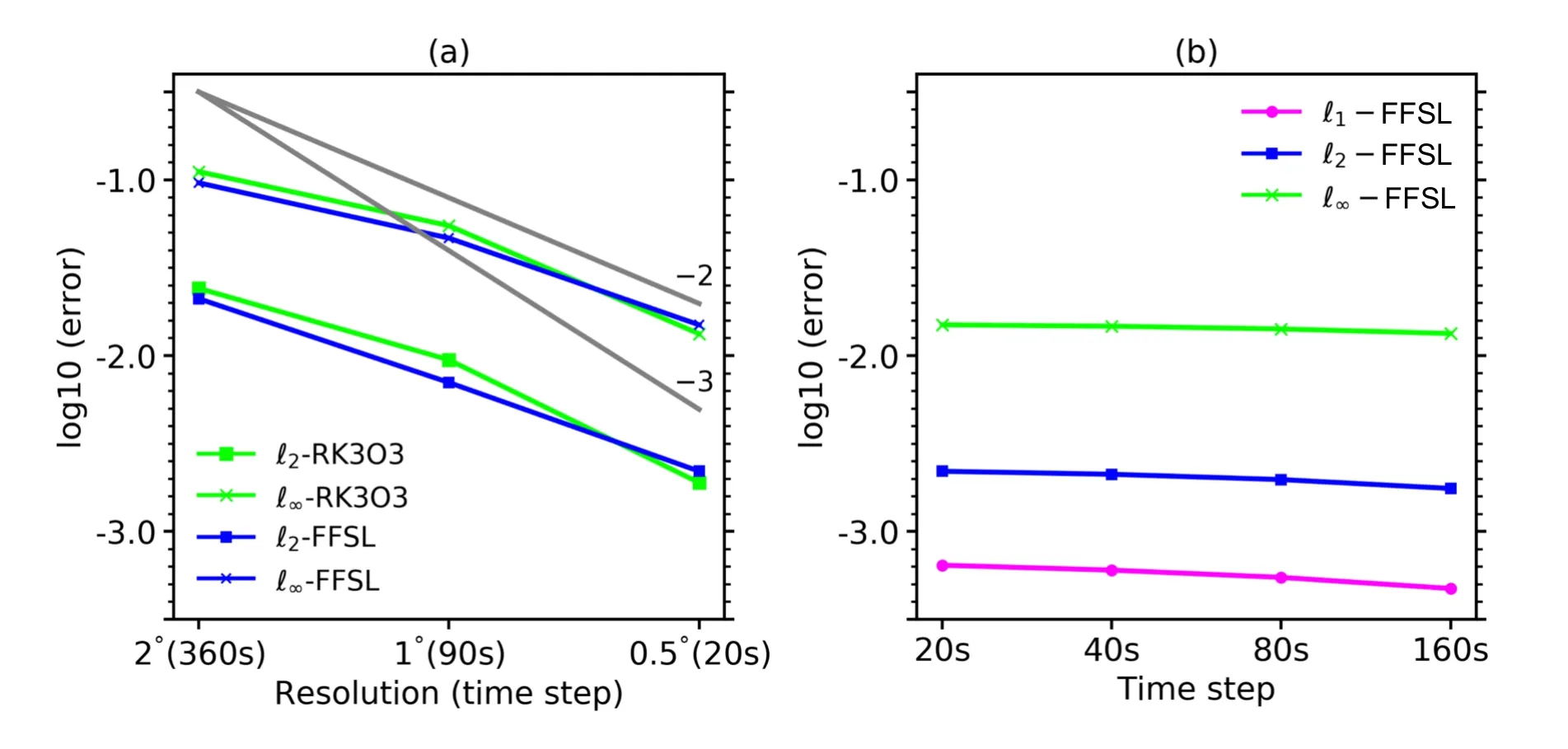
Fig.6.Error norms in the test case of the two-dimensional moving vortex.Panel (a) shows the convergence rates ofℓ2 and ℓ∞ for the limited variations of the RK3O3 and FFSL schemes.The error norms of the FFSL with a fixed resolution of 0.5º and variable time-step sizes are displayed in panel (b).

Fig.7.The horizontal cross-sections of tracer q3 at 4900 m on model day 6 of the DCMIP 1-1 three-dimensional deformational flow test.Two horizontal (FFSL and RK3O3) and two vertical (PPM and RK3O3) flux operators are used in the transport model.The resolution is 1º with 60 vertical levels.White areas show numerical undershoots.The minimum(min) and maximum (max) of each simulation are also shown in each panel.

Fig.8.As in Fig.7 but for t=12 days.

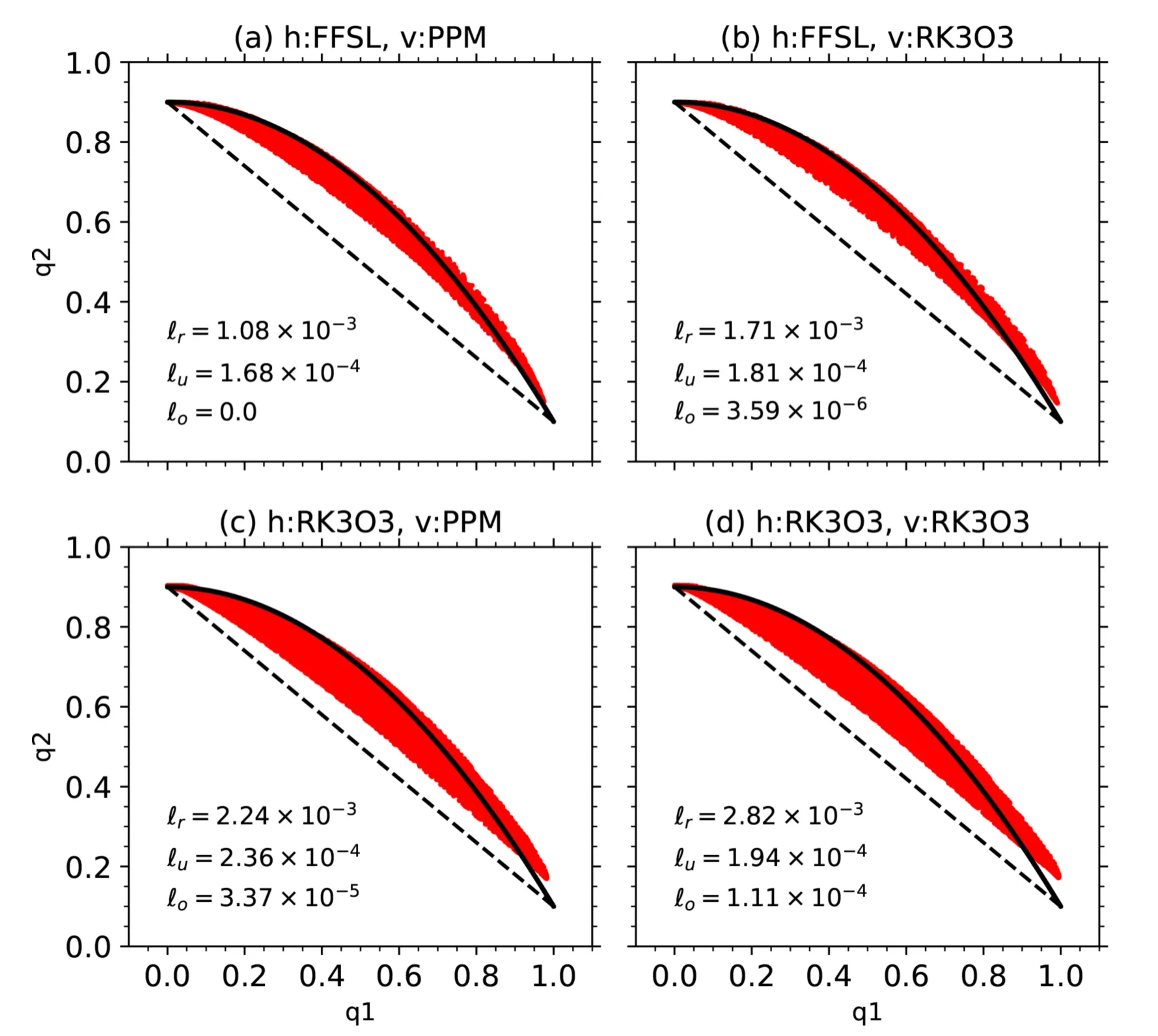
Fig.9.Scatter plots of two nonlinearly correlated tracer fields,q1 and q2,in the five vertical levels around a height of 4900 m at t=6 days.The mixing diagnostics ℓr,ℓu,and ℓo are calculated for each combination of two horizontal flux operators (FFSL and RK3O3) and two vertical flux operators (PPM and RK3O3).

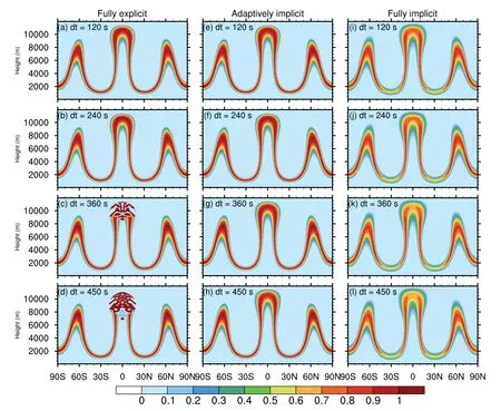
Fig.10.The three-dimensional Hadley-like meridional circulation test (DCMIP1-2): latitude–height plot at the longitude of 180ºat 12 h with four time-step sizes (from the upper rows to bottom rows: 120 s,240 s,360 s,450 s) using (a–d) fully explicit,(e–h)adaptively implicit,and (i–l) fully implicit vertical advection schemes.There are 180 vertical levels with a horizontal resolution of 1º.

Fig.11.As in Fig.10 but at 24 h.

To further assess the robustness of the adaptively implicit vertical algorithm,we calculate the convergence rates from the Hadley-like circulation test.The resolutions are set to 2◦L90,1º L180,and 0.5º L360 with time-step sizes of 720 s,360 s,and 180 s,respectively,to trigger the adaptively implicit algorithm.The two horizontal flux operators and two vertical flux operators are combined to form four configurations.In addition,the monotonic slope-limiter is used in the PPM-based solvers,and the FCT flux limiter is also applied in each sub-step of the RK3 time integrator.

As seen in Fig.12,all four combinations produce similar results in which the error norms converge between the first and second order,which is somewhat lower than those given in Kent et al.(2014).This is reasonable because the vertically implicit solver uses a first-order upwind algorithm.On the other hand,simple operator-splitting is used in the horizontal–vertical coupling.In addition,the numerical accuracy is also reduced by the non-uniform vertical spacings of the vertical coordinate.The RK3O3-based solvers exhibit marginally higher convergence rates than the PPM-based solvers do,and they are the same as the convergence rates in the two-dimensional solid-body rotation test (shown in Fig.4).There are only minor differences among the four combinations in terms of ℓ1,ℓ2,ℓ∞.In general,the PPM-based three-dimensional solvers produce fewer errors than the RK3O3-based solvers do at each resolution,particularly for 2º L90 and 1º L180.Overall,the outcomes are insensitive to the combination of two horizontal flux operators and two vertical flux operators,which further demonstrates the robustness of the three-dimensional tracer transport model.These results are consistent with the results of the previous threedimensional deformational flow test cases.

Fig.12.The three-dimensional Hadley-like meridional circulation test: numerical error norms of ℓ1,ℓ2,ℓ∞ for the (a)PPM-based and (b) RK3O3-based vertically explicit transport solvers,with two horizontal transport schemes of FFSL and RK3O3.The gray lines denote the ideal first-and second-order convergence rates.

4.Conclusions

This study developed a three-dimensional tracer transport model on a regular latitude–longitude grid.The model maintains its computational stability in the presence of large Courant numbers.The model uses a flux-form conservation tracer equation,and the key is the flux computation on the mesh interface.To enable a high Courant number along the zonal direction within the scheme,an FFSL scheme is chosen as the horizontal solver.An adaptively implicit vertical advection scheme is applied to enhance the stability of the vertical discretization.For comparison,we adopted a third-order upwind advection scheme with the RK3O3 scheme in the horizontal and vertical directions as a reference.

For the two-dimensional test cases,the FFSL scheme with a slope-limiter is comparable to or better than the RK3O3 scheme with FCT in terms of accuracy and monotonicity.Furthermore,the FFSL scheme allows for much larger time-step sizes than does the RK3O3 scheme.The horizontal FFSL scheme in conjunction with the vertical PPM scheme is demonstrated to be the best configuration in terms of accuracy,monotonicity,and computational efficiency in the three-dimensional advection tests.The stringent Courant number constraint can be alleviated via the adaptively implicit vertical advection algorithm,allowing the time-step size to be increased.

The three-dimensional tracer transport model has been implemented in the global atmospheric baroclinic dynamical core we are developing,and only the tracer transport module was evaluated in this work.Further work on the coupling of the tracer transport module and the dynamical core with one or two physics packages may be available in the near future.Additionally,the use of the incremental remapping method and the floating Lagrangian vertical coordinate presents promising alternatives that are not constrained by the vertical Courant number.Further exploration can be pursued in these areas for future research.

Acknowledgements.This work was jointly supported by the National Natural Science Foundation of China (Grant No.42075153) and the Young Scientists Fund of the Earth System Modeling and Prediction Centre (Grant No.CEMC-QNJJ-2022014).

Data availabilitystatement.Data for this study are available from the first author upon request.

APPENDIX A

A Minor Error in the Monotonicity Constraints for the PPM in Lin (2004)

In order to ensure monotonicity,a slope limiter is required in the FFSL transport scheme.Constraining the slope or mismatch is a critical process.In Appendix B of Lin (2004),there is a minor error in Eq.(B1) for constraining the mismatch.The correct formulation is

where ∆qiis the “mismatch” that represents the difference betweenqi+1/2andqi-1/2for theith cell.The superscript“mono” denotes the final value used for monotonicity.The superscripts “min” and “max” denote the values needed in the calculation,as in Lin (2004).The functions “sign”,“min”,and “max” are as defined in the Fortran language as in Lin (2004).