Haijin DAI and Qiang YAO

College of Meteorology and Oceanography, National University of Defense Technology, Changsha 410073, China

ABSTRACT How atmospheric and oceanic circulations respond to Arctic warming at different timescales are revealed with idealized numerical simulations.Induced by local forcing and feedback, Arctic warming appears and leads to sea-ice melting.Deep-water formation is inhibited, which weakens the Atlantic Meridional Overturning Circulation (AMOC).The flow and temperature in the upper layer does not respond to the AMOC decrease immediately, especially at mid-low latitudes.Thus, nearly uniform surface warming in mid-low latitudes enhances (decreases) the strength (width) of the Hadley cell (HC).With the smaller northward heat carried by the weaker AMOC, the Norwegian Sea cools significantly.With strong warming in Northern Hemisphere high latitudes, the long-term response triggers the “temperature-wind-gyretemperature” cycle, leading to colder midlatitudes, resulting in strong subsidence and Ferrel cell enhancement, which drives the HC southward.With weaker warming in the tropics and stronger warming at high latitudes, there is a stronger HC with decreased width.A much warmer Southern Hemisphere appears due to a weaker AMOC that also pushes the HC southward.

Key words: Hadley cell, Arctic amplification, Southern Hemisphere warming, Atlantic Meridional Overturning Circulation Citation: Dai, H.J., and Q.Yao, 2023: Role of ocean dynamics in the seasonal Hadley Cell: A response to idealized Arctic Amplification.Adv.Atmos.Sci., 40(12), 2211-2223, https://doi.org/10.1007/s00376-022-2057-7.

1.Introduction

Over the past several decades, surface air temperature(SAT) has increased globally as a result of anthropogenic greenhouse gas emissions (mainly the concentration of carbon dioxide, CO2; Forster et al., 2021).Due to local forcing and feedback (Stuecker et al., 2018), SAT increases much faster in the Arctic than in other regions, resulting in Arctic-amplified warming (Serreze and Francis, 2006; Screen and Simmonds, 2010).Some studies (Graversen et al., 2014; Dai,2021) estimate that surface albedo feedback from sea-ice loss contributes as much as 40% and dominates the local forcing and feedback.A further study reveals that increased solar radiation absorption induced by sea-ice loss has caused significant Arctic Ocean warming in summer (He et al., 2018), but the simultaneous warming in the Arctic atmosphere is less significant, since the Arctic atmospheric temperature in summer is much higher than that in the ocean(Chung et al., 2021).Typically, the Arctic Ocean absorbs(releases) heat in the warm (cold) season, which maintains a steady annual cycle.Thus, additional heat storage would be released in the cold season with smaller insulation by sea ice (Dai et al., 2019), as well as stronger vertical mixing induced by more water freezing.In addition, CO2prevents longwave radiation from escaping to outer space and warms the surface, especially in winter.Planck feedback (surface temperature) is negative and smaller than that in the tropics(Pithan and Mauritsen, 2014).Water vapor (positive feedback) makes little contribution to Arctic warming because of the low amounts over the Arctic (Walsh, 2014; Jenkins and Dai, 2021).Some studies also consider lapse rate feedback to be important for Arctic amplification because little heat is transported upward in a stable atmosphere (Goosse et al., 2018).Clouds provide different contributions to Arctic warming depending upon their height and type (Huang et al.,2017), although the impacts are relatively small (Jenkins and Dai, 2021).Eventually, seasonal Arctic warming reaches its maximum and minimum in the cold season and warm season, respectively (Dai, 2021).

With a warmer Arctic [in a long Greenhouse Gas(GHG) induced warming simulation], Arctic low pressure deepens, which enhances the meridional pressure gradient between the Arctic and midlatitudes and strengthens, the westerly flow, which can better trap the cold air in the Arctic(Dai and Song, 2020).Previous studies (Dai and Deng,2022) suggested recent cold outbreaks may be related to internal multidecadal variations amplified by ice-air interaction over the Arctic Ocean.Besides, winter daily temperature variability over northern mid-high latitudes will decrease under GHG-induced warming mainly due to reduced meridional temperature gradients (Chen et al., 2019; Dai and Deng,2021).The strengthened westerlies may lead to increased planetary wave activity (Blackport and Screen, 2020).This maintains a seesaw pattern of winter precipitation variability between North China and the southwest United States via the East Asian trough and North American high (Dai et al.,2021); this seesaw pattern is also maintained in summer,although the dominant mechanism becomes the subtropical high, whose location is determined by the subsidence branch of the Hadley cell.On the other hand, an important teleconnection is brought out as a “pole-to-pole” mechanism, which describes how Arctic warming influences Antarctica through the Hadley cell and the Ferrel cell (Shin and Kang, 2021).Thus, the Hadley cell becomes an important medium for Arctic amplification to influence other regions.

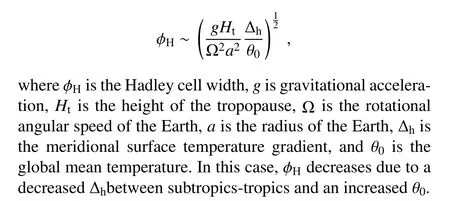
Previous studies (Held and Hou, 1980; Lu et al., 2007)have asserted that the meridional surface temperature gradient, tropopause height, angular velocity of the Earth, radius of the Earth, gravitational acceleration of the Earth, and global mean temperature determine the strength and position of the Hadley cell.Although mid-low latitude warming in recent years has been dominated by internal variability,such as the El Niño-Southern Oscillation and the interdecadal Pacific oscillation/Pacific decadal oscillation, external forcings have become the dominant factors in long warming simulations.Mid-low latitude warming may be induced by both remote forcings (i.e., Arctic amplification; Dai et al., 2021;Shin and Kang, 2021) and local forcing and feedback (i.e.,Planck feedback, water vapor feedback, and cloud feedback).Thus, it is necessary to separate the Hadley cell variability induced by Arctic amplification from that induced by local warming.

Shin and Kang(2021) proposed an important mechanism regarding significant Arctic warming/cooling in slab ocean experiments.The results are consistent with previous studies(Lu et al., 2007) showing that the Hadley cell strengthens(weakens) and shifts northward (southward) on a decadal scale during Arctic warming (cooling).A question to consider is: Do ocean dynamics play any role in Hadley cell evolution or can Hadley cell anomalies be achieved without ocean dynamics?

In this study, we explore how the Hadley cell evolves toward surface forcing variation, which is a result of ocean dynamics at different timescales in response to different external forcing scenarios.First, we determine the ocean response to Arctic warming on different timescales, since the spin up of deep water ocean circulation (i.e., Atlantic Meridional Overturning Circulation, AMOC) requires a period of decades or even longer.Second, we seek to understand how the Hadley cell responds to ocean dynamics on different timescales, especially on a longer timescale.Third,we compare the response of the Hadley cell to Arctic-amplified warming from the Hadley cell response to increased CO2forcing.To address these problems, this paper is organized as follows: the coupled model and perturbation experiments are introduced in section 2.We analyze the results from the polar albedo forcing experiment in section 3.A summary and discussion are provided in section 4.

2.Model and experiments

To obtain Arctic amplification, a fully coupled global climate model, the Community Earth System Model (CESM)version 1.0 (CESM1.0; Hurrel et al., 2013), is used in this study.Here, we employ a model grid of T31_gx3v7, which consists of a spectral atmosphere model (Community Atmosphere Model version 5, CAM5; Neale et al., 2012), a land model (Community Land Model version 4, CLM4;Lawrence et al., 2012), a tripolar grid ocean model (Parallel Ocean Program version 2, POP2; Smith et al., 2010), and an ice model (Community Ice CodE version 4, CICE4; Hunke and Lipscomb, 2008).T31 (triangular-cubic spectral truncation) has a horizontal resolution of 3.75° (though we suggest that to simulate the modern day climate, the horizontal resolution should be better than 2º) in CAM5 and CLM4, where CAM5 has 26 vertical layers.The gx3v7 is a nominal 3°grid in the horizontal direction with the North Pole displaced to land in POP2 and CICE4, although POP2 also has 60 vertical layers.We have completed many studies (Yang and Dai,2015; Dai et al., 2017, 2021; Dai, 2021) with this model before.

With CESM1.0, we complete a 2000-year control run(CTRL), a 500-year CO2perturbation run (2xCO2) and a 500-year surface albedo-perturbation run (0.1A).The CO2concentration is set to 285 ppm (no increased CO2forcing)in CTRL and 0.1A.In previous studies, we obtained a quasiequilibrium climate status after a 1000-year integration in CTRL (Yang and Dai, 2015).We continued to integrate the CTRL for another 1000 years (year 1001-2000) under equilibrium status (Dai et al., 2017) and used the last 500 years as a climate reference.In the surface albedo-perturbation run,the sea ice albedo is artificially set to 10% of its original value (without changing the albedo of the land ice albedo or other parts in the coupled model), which greatly decreases the surface albedo of the ice-covered ocean globally.In contrast, there is no artificial revision in surface albedo in the 2xCO2 experiment, in which the CO2concentration increases by 1% per year in the first 70 years and then remains constant at a concentration of 570 ppm in the following integration.Both 0.1A and 2xCO2start from the year 1500 in CTRL and integrate for 500 years separately(Fig.1).

Fig.1.Flow chart of the numerical experiment used in this study.The preindustrial scenario (B1850) is simulated with CESM T31_gx3v7.The control experiment(CTRL) is integrated over 2000 years, although it nearly reaches equilibrium at the 1000th year.In the 2xCO2 experiment, the concentration of CO2 increases by 1% in the first 70 years; when the CO2 concentration reaches twice the original amount, it stops increasing.In the 0.1A experiment, the ice albedo (to shortwave radiation) is set as 0.1 times its original value.Two sensitivity experiments are integrated parallel to 1501-2000 in CTRL.

There are several reasons we made comparison between the 0.1A experiment and 2xCO2experiment.Although CO2concentration has linearly increased over recent centuries (which is also set in 1501-1570 in 2xCO2experiment), Arctic warming and sea-ice loss have mainly occurred only since 1980 (not shown), which may suggest that surface albedo feedback (as well as decreased insulation in winter) induced by sea-ice loss instead of CO2forcing has become the key mechanism for Arctic warming in recent decades (thus, the 0.1A experiment can partly reflect recent climate change).On the other hand, results from the 0.1A experiment are considered as pure response to the polar warming (there is nearly no change in mid-low latitude at the beginning), while results from the 2xCO2experiment are considered as current climate change (although not so accurate as the CMIP6).If the Hadley cell in the 0.1A experiment is consistent with that in the 2xCO2experiment, we conclude that the Hadley cell response to Arctic warming dominates/plays an important role in current Hadley cell anomaly.Otherwise, the 0.1A experiment may offer a possible scenario if Arctic keeps rapidly warming in the future.The coupled climate model offers a monthly mean output in this study.The climate anomalies in the 0.1A or 2xCO2experiment are obtained by subtracting the corresponding states in the CTRL.Triggered by different mechanisms, Arctic amplification is achieved in both idealized scenarios (0.1A and 2xCO2experiment), although surface warming is larger in 0.1A experiment due to extremely large solar radiation absorption at surface (reduced surface albedo).On the other hand,seasonality of Arctic surface warming in 0.1A experiment is nearly the same as that in 2xCO2experiment, both of which reach their minimum and maximum in summer and autumn,respectively, and their second peak in spring.In this study,we focus on both the transient responses and the equilibrium responses (this definition is created according to temperature in the 0.1A experiment (section 3).We applied this definition to the 2xCO2experiment for better comparison with 0.1A experiment), which are the seasonally/annually averaged fields over the first 20-year integration and 301-500 years integration, respectively, unless stated otherwise.

3.Hadley cell evolution under warming conditions in the Arctic

Fig.2.Temporal changes in (a) globally integrated annual net radiation flux (black), net downward solar radiation (royal blue), and net outgoing longwave radiation (red) at the TOA(positive for downward anomaly; W m-2), zonally averaged annual (b) sea surface temperature anomaly (units: °C) and (c)surface air temperature anomaly (units: °C) in the 0.1A experiment.

Although no increased CO2forcing is added in the CTRL and 0.1A experiments, AA is still achieved in the 0.1A experiment compared with the results in the CTRL experiment.Due to artificially decreased surface albedo, additional solar radiation is absorbed, which leads to net radiation addition at the top of atmosphere (Fig.2a).Arctic surface warming (Fig.2c) is achieved by additional solar radiation absorption induced by sea-ice loss (Fig.1a in Dai, 2021).Influenced by ocean dynamics at different timescales, the sea surface temperature (SST) anomaly exhibits different spatial patterns in the first 20 years (positive SST anomaly in subpolar in NH), 21-300 years (positive SST anomaly equatorward expansion in mid-high latitude of SH) and 301-500 years (no significant change in SSTA Fig.2b), which are defined as the early-transient stage, late-transient stage and equilibrium stage, respectively.Although SST in the 2xCO2 experiment evolves on different timescales (the early transient stage in 2xCO2 ends by the 80th year, while the equilibrium stage of 2xCO2 here is actually during the middle period of stage I in Yang et al., 2018; Fig.A1 in the Appendix), we still use the definition above for a better comparison.We also found that the stage definition is consistent with the features of AMOC index (rapid decrease, slow decrease and no obvious trend) in the 0.1A experiments (blue line in Fig.1b in Dai et al., 2021).In this study, the mechanisms of surface warming in the early-transient stage and equilibrium state are revealed in section 3.1 and section 3.2, respectively.The corresponding anomalies in the Hadley cell and possible consequences are also studied, together with the potential influence of multiple-scale ocean dynamics.

3.1.Hadley cell response to Arctic warming

In the 0.1A experiment, surface albedo over the ice-covered region is decreased artificially, and additional solar radiation is absorbed at the surface, especially in summer (approximately 67.4 W m-2in the first 20 years).The additional solar radiation absorption is stored as seasonal heat storage in the subsurface ocean during summer and released to the atmosphere in autumn-winter (not shown), which leads to Arctic warming (66°-90°N) reaching its minimum (0.8°C) and maximum (2.3°C) in the warm season and cold season, respectively.Sea-ice melt (Fig.3a, black line; different from current climate studies (Dai, 2022; Deng and Dai, 2022) in which annual sea-ice changes little) induced by Arctic warming produces freshwater (Fig.3a, blue line) and decreases the water density in the North Atlantic (Fig.3a, red line; Fig.1a in Dai et al., 2021b), which inhibits deep-water formations and decreases AMOC from 22 Sv to 18 Sv in the first 20 years(nearly 20%; Fig.1b in Dai et al., 2021).Following Yang et al., 2015, the meridional overturning circulation (MOC) and the associated heat transport are partitioned into Euler mean circulation, circulation induced by mesoscale eddies (Bolus term) and submesoscale eddies (submeso term) as well as a diffusion term.Although the results show that the MOC decreases significantly in the first 20 years, the meridional oceanic heat transport (OHT; Fig.3b blue line) anomaly is mainly contributed by mesoscale processes (Fig.3c short dash line) both in the Northern Hemisphere (NH) and Southern Hemisphere (SH), which is much larger than the contribution from mean circulation (Fig.3c long dash line).Similar local forcing and feedback also occurred in the Antarctic region and resulted in surface warming in the high latitudes of the SH (Fig.2c), which decreased the meridional temperature gradient and eastward wind.

Both the equatorward wind-driven Ekman transport(Fig.4c) and poleward eddy-induced circulation decrease in the Deacon cell, although the former dominates the Deacon cell anomaly and pushes it equatorward (Fig.4b shading).In turn, the weakened Deacon cell decreases the subtropical cell, especially in the Pacific-Indian Ocean (Fig.4c).The circulation anomaly mainly occurs in the lower layers, and mesoscale processes dominate the heat transport anomaly(0.5 PW at 30°S; 1PW=1012W; Fig.3b blue line).Arctic warming expands equatorward (as far as 50°N, Fig.3b green line), and less poleward transport also warms the lower layers (approximately 1.0°C in the upper 500 m; Fig.4a,shading).In this stage, the temperature profile (Fig.4a shading) and upper-layer current (Fig.4b shading) remain nearly unchanged at mid-low latitudes.As a result, there is no significant warming at the surface at mid-low latitudes (Fig.3b green line).Since there is strong (weak) warming in polar regions (mid-low latitude), AA appears.

Fig.3.(a) Zonally integrated ice-covered area anomaly (black line, units: 105 km2), zonally averaged sea surface salinity anomaly (blue line, units: PSU), and sea surface density anomaly (red line, units: kg m-3) in the 0.1A experiment.(b)Oceanic heat transport (OHT) anomaly (blue line, unit: PW,1PW=1012 W), atmospheric heat transport anomaly (red line,units: PW), total meridional heat transport anomaly (black line,units: PW) and zonal mean surface air temperature anomaly(units: °C) in 0.1A are shown in (b).(c) OHT anomaly partitioned into Eulerian (long dash), Bolus (short dash),submesoscale and diffusion terms, two of which are shown,PW).The results are annual anomalies over the first 20 years in the experiments with a confidence level of 95% (Student’s ttest).

Fig.4.(a) Vertical profile of the temperature anomaly(shading, °C) in the Global Ocean and the climate mean temperature (contour).(b) Streamfunction of the global meridional overturning circulation anomaly in the 0.1A experiment is shown and the climate mean in the CTRL(contours, Sv.) (c) is the same as (b) but for the Eulerian part in the Pacific-Indian Ocean.All anomalies are shown at the 95%confidence level (Student’s t-test).

On the other hand, the meridional temperature gradient remains unchanged at low latitudes, as do the easterlies (via the thermal wind) and the subtropical cell (STC; anomaly is smaller than 1%) it drives (via Ekman transport) in the NH.The NH Hadley cell increases slightly (1%-2.4%; Figs.5a,c) in spring and autumn, while it decreases slightly (1%-2%; Figs.5e, g) in summer and winter.As a result, the strength of the annual mean Hadley cell in the NH remains nearly unchanged in the first 20 years (red line in Fig.1b in Dai et al.2021; seasonal Hadley cell anomalies in the early transient stage in 2xCO2 are also shown for comparison in Figs.5b, d, f, h).This result is similar to the meridional atmospheric heat transport (AHT) at low latitudes (Fig.3b, red line).Strong (weak) warming at high (mid) latitudes decreases the meridional temperature gradient (-), which decreases the zonal wind via the thermal wind.In turn,weaker westerly (jet shear) decreases the eddy activity (via barotropic instability) and meridional AHT (approximately 0.17 PW and 0.2 PW in the NH and SH, respectively; Fig.3b red line).The strong warming in the Arctic also inhibits local subsidence and decreases the Polar cell, which in turn decreases the Ferrel cell at mid-high latitudes.As a result,the Hadley cell moves northward, except in winter (Table 1).In addition, the SH Hadley cell also strengthens slightly (0%-3% in each season, Table 1).The width of the NH Hadley cell can be explained via the Hadley cell expansion estimate(Held and Hou, 1980; Lu et al., 2007)

Fig.5.The seasonal atmospheric meridional mass streamfunction in the CTRL (contour) and differences between the sensitivity experiments and the CTRL (shading), taken from the first 20-year numerical results (109 kg s-1).

This anomalous Hadley cell pattern is also achieved in a slab ocean experiment, which displays the result of ocean dynamics as a surface forcing (Shin and Kang, 2021),although the polar warming here is much larger than that due to the extremely high amount of solar radiation absorption.The results suggest that even though the AMOC decreases due to continuing sea-ice melt, the surface temperature at low latitudes does not respond immediately, while the Hadley cell moves northward due to Arctic warming.

3.2.Toward a hemispheric energy adjustment

In the following two stages, we find that the vertical profile of the global oceanic temperature anomaly is consistent with that of the temperature anomaly in the Atlantic Ocean(Fig.6a, shading).Response timescale analysis is applied to the vertical profile of oceanic temperature (Fig.6a) to determine the sequence of ocean dynamics.Here, we define the response timescale as the beginning of a period in which the temperature anomaly always reaches 70% of that in the equilibrium state [following Yang and Zhu (2011), in the 2xCO2 experiment, we took the last two centuries as equilibrium for comparison, but it is during the middle period of stage I in Yang et al.(2018)].The result of the response timescale analysis (Fig.6a) suggests that the first region to reach equilibrium is the polar region [90°-60°S, 60°-90°N],followed by the thermocline in mid-low latitudes.The sea surface temperature in mid-high latitudes [30°-60°N] reached equilibrium slightly earlier than the sea surface temperature in the tropics.Based on the timescale analysis above, the implication in the last two stages is described as follows:warming at high latitudes decreases the meridional temperature gradient, which in turn decreases the westerly at the surface via the thermal wind.As a result, cyclonic wind stress decreases (Fig.6c) and induces a weaker southward gyre via the Sverdrup relation.Due to mass conservation, the western boundary current decreases, especially in the region of 30°-40°N.Without warm water being transported poleward and sinking at high latitudes, there is significant cooling(approximately 4°C) in the region of approximately 60°N(Fig.6b; Figs.8a, c, e, g).The cooling (warming) at mid(low) latitudes in the NH enhances the meridional temperature gradient (-) and decreases the westerlies at the surface via the thermal wind.As a result, more heat is trapped at low latitudes, resulting in warming in the tropics, as well as weaker surface westerly (Fig.6c).Then, the STC as well as the Walker circulation are weakened, and more heat is stored in lower layers and in the eastern part of the oceans (Fig.6a shading).On the other hand, with surface warming in the Antarctic region, sea ice melts and freshens the surface ocean, which inhibits bottom water formation.As a result,there is significant warming at high latitudes in the SH(Fig.6b; Figs.8a, c, e, g).

During the equilibrium state, the OHT decreasesmainly due to a weaker mesoscale process, which is larger than the mean circulation contribution.Thus, we conclude that OHT anomalies occur mainly due to mesoscale processes.Strong cooling at 30°-40°N (Fig.6b; Fig.8a, c, e, g shading) largely enhances the subsidence branch there (as well as the Ferrel cell; Figs.9a, c, e, g); thus, the edge of Hadley cell moves equatorward (Table 2).On the other hand, the enhanced warming in the tropics increases the convection in the Hadley cell.As a result, the strength of the Hadley cell grows, although the expansion of the Hadley cell is eliminated (nearly no cold color in NH; Fig.9a, c, e,g shading).The strengthened Hadley cell increases the AHT everywhere, except in the region of 40°N-90°N, where the eddy activity decreases due to a smaller meridional temperature gradient.

Table 1.The seasonal variation in the Hadley cell in the first 20 years in each experiment is presented in this table.N and S indicate the north and south branches of the Hadley, respectively, and stren and mid indicate the strength and the ITCZ at 500 hPa, respectively.For the Hadley cell strength, a positive (negative) value means mass transport northward (southward), in 109 kg s-1.For the Hadley cell location, a positive (negative) value means that the location is in the Northern (Southern) Hemisphere.

Fig.7.Same as in Fig.6 but for the results from the 2xCO2 experiment.

Without strong Arctic warming (Figs.7a, b; Figs.8b, d,f, h shading) induced by artificially decreased surface albedo, there is little meridional temperature gradient between 30°N and 50°N in the 2xCO2 experiment (Fig.7b Figs.8b, d, f, h shading).Thus, the wind curl (Fig.7c vector)and horizontal gyre remain strong (Fig.7c shading).On the other hand, a decreased AMOC prevents warmer water vapor transport poleward at high latitudes in the NH.Thus,cooling (warming) occurs at approximately 60°N (at 30°-40°N).On the other hand, an increased CO2forcing also induces warming globally due to the greenhouse effect(Figs.8 b, d, f, h).In the 2xCO2 experiment, the sea surface warming in the SH (Fig.7b shading) exhibits a similar pattern as that in the 0.1A experiment (Fig.6b, shading), which suggests that the sea surface warming in the SH is mainly a result of the AMOC decreasing instead of a local forcing.Without a slow adjustment (temperature-wind-gyre-temperature) between 30°N and 40°N, the temperature reaches equilibrium much faster (Fig.7a, contour), as does the sea surface temperature in the tropics.On the other hand, enhanced warming in the tropics (due to feedback of water vapor and clouds; Figs.8b, d, f, h) suggests stronger convection and Hadley cell, while warming at midlatitudes and weaker warming at high latitudes in the NH suggest that the subsidence branch may move poleward (blue color is in the NH;Figs.9a, h, shading; Table 2).As a result, the Hadley cell strengthened and expanded poleward in the 2xCO2 experiment (Figs.9b, d, f, h; Table 2).

Fig.9.Same as in Fig.4, but results from the last two centuries.

4.Conclusions and discussion

This study investigated “how Arctic-amplified warming influences the surface temperature and large-scale atmospheric circulation at mid-low latitudes” with a coupled climate model.Although the sensitivity experiments are idealized, they can realistically reflect the climate change in the real world.Triggered by different mechanisms, Arctic warming in 0.1A experiment is mainly induced by reduced surface albedo, while the Greenhouse effect and surface albedo feedback are the main mechanisms in 2xCO2 experiment.Furthermore, Arctic warming in these two scenarios share similar seasonality, which ensures the reasonability of the following comparison.

In this study, we found that most of the seasonal atmospheric circulation exhibits a similar trend as the annual atmospheric circulation, especially in an equilibrium state.We discuss the atmospheric circulation response to a greater extent in several ways.

First, Arctic warming rapidly decreases the AMOC,mainly flowing in the lower layers.However, surface temperature adjustment is mainly completed by circulation in the upper layers.In our experiments, the temperature in the polar region reaches equilibrium first, then the thermocline temperature at mid-low latitudes.The temperature in the wind-driven gyre can reach equilibrium after the “temperature-wind-gyre-temperature” cycle runs over a long period.Mesoscale processes dominate the meridional OHT anomaly instead of Eulerian (mean) circulation, which suggests that mesoscale processes may dominate the temperature response to the AMOC anomaly.This conclusion demonstrates the importance of understanding and realistically simulating oceanic mesoscale processes in numerical climate models.In addition, the similar pattern of surface temperature anomalies in the SH in the two experiments with and without strong Arctic warming and surface albedo decrease confirms that the long-term response of surface temperature in the SH is mainly controlled by the AMOC anomaly.

Second, three features (strength, width, and location) of the Hadley cell are studied in this manuscript.The strength of the Hadley cell in our experiment seems to be consistent with the strength of the ascending branch, both of which are maintained by the tropical surface temperature.The numerical results suggest that as the tropical surface temperature increases, whether it is caused by Arctic warming or additional CO2forcing, the ascending branch and the Hadley cell strengthen.The meridional temperature between high and low latitudes and the averaged surface temperature seem to dominate the width of the Hadley cell in our experiments.Thus, extreme warming at high (low) latitudes may decrease (increase) the Hadley cell width.The location of the Hadley cell can be pushed northward (southward) due to strong warming at mid-high latitudes in the NH (SH).

Third, a comparison is made with and without increased CO2forcing (surface albedo decrease) in the numerical experiments.The results show that before the surface temperature and circulation in the upper layer respond, the surface warming at midlatitudes is weak (compared with Arctic warming) and nearly uniform.Thus, the Hadley cell strengthens and moves northward in both scenarios.As a long-term response to Arctic warming and decreased AMOC, cooling at midlatitudes strengthens the subsidence branch and the Ferrel cell, thus pushing the Hadley cell edge equatorward.The results from the 2xCO2 experiment are more consistent with the recent climate status, which exhibits a stronger poleward expansion of the Hadley cell.However, this study also warns that an extremely warm high latitude led by surface albedo feedback (sea ice loss)may induce colder temperatures at midlatitudes, as well as a stronger but narrower Hadley cell.Based on the results of this study, we suggest that ocean dynamics should be considered when studying the Hadley cell.

Table 2.Same as in Table 1 but for the Hadley cell in the equilibrium state.

Another issue is related to the pole-to-pole teleconnection, which is an important mechanism for the Antarctic response to Arctic amplification.Shin (Shin and Kang,2021) demonstrated how the Antarctic is warmed solely according to atmospheric circulation in the Arctic warming scenario, while we found that ocean dynamics (due to AMOC weakening) may also warm the Antarctic.Thus, the Antarctic has experienced little warming in recent decades,which seems to be unreasonable and will be studied in our future work.

Acknowledgements.We are grateful to Dr.Qin WEN for the valuable suggestions.

APPENDIX

Fig.A1.Zonally averaged monthly sea surface temperature anomaly in 2CO experiment (°C).