Lanying CHEN, Renhao WU, Qi SHU, Chao MIN, Qinghua YANG, and Bo HAN*

1School of Atmospheric Sciences, Sun Yat-sen University, and Southern Marine Science and Engineering Guangdong Laboratory (Zhuhai), Zhuhai 519082, China

2First Institute of Oceanography, Ministry of Natural Resources, Qingdao 266061, China

ABSTRACT This study assesses sea ice thickness (SIT) from the historical run of the Coupled Model Inter-comparison Project Phase 6 (CMIP6).The SIT reanalysis from the Pan-Arctic Ice Ocean Modeling and Assimilation System (PIOMAS)product is chosen as the validation reference data.Results show that most models can adequately reproduce the climatological mean, seasonal cycle, and long-term trend of Arctic Ocean SIT during 1979–2014, but significant intermodel spread exists.Differences in simulated SIT patterns among the CMIP6 models may be related to model resolution and sea ice model components.By comparing the climatological mean and trend for SIT among all models, the Arctic SIT change in different seas during 1979–2014 is evaluated.Under the scenario of historical radiative forcing, the Arctic SIT will probably exponentially decay at –18% (10 yr)–1 and plausibly reach its minimum (equilibrium) of 0.47 m since the 2070s.

Key words: sea ice thickness, Arctic Ocean, climate change, historical simulation, CMIP6

1.Introduction

Sea ice is a significant component of the Arctic environment (Parkinson and Cavalieri, 2008).It can modulate the global atmosphere and ocean circulation mainly by changing heat, momentum, and moisture exchanges between the atmosphere and ocean (Sévellec et al., 2017; Mallett et al., 2021).Arctic sea ice is one of the crucial indicators of global climate change (Notz et al., 2016; Serreze and Meier, 2019).With ongoing global warming, sea ice has retreated dramatically in the Arctic Ocean (Stroeve et al., 2012a, b; Kwok and Cunningham, 2015), which has a significant impact on local ecosystem evolution (Post et al., 2013; Divoky et al., 2015),navigation (Smith and Stephenson, 2013; Melia et al., 2016;Min et al., 2022a, b), and resource extraction (Meier et al.,2014; Petrick et al., 2017).

Sea ice thickness (SIT) is one of the most important physical properties of the cryosphere as it directly modulates the energy exchange efficiency between the adjacent ocean and atmosphere.Among the existing observations, field observations, including sea ice draft measurements from submarine upward-looking sonar (ULS), moored ULS, Ice Mass Balance(IMB) buoys, and airborne electromagnetic measurements,are a common way to derive Arctic SIT (Schweiger et al.,2011).Additionally, draft observations from submarines and moorings are converted to ice thicknesses using an ice density of 928 kg m–3, and the snow water equivalent estimated by the model and uncertainty in the draft-to-thickness conversion is relatively small (<10%) (Schweiger et al.,2011).The maximum uncertainties of the laser altimetry data from satellites, like ICESat and ICESat-2, were estimated to be 0.5 m for individual 25-km ICESat grid cells (Kwok et al., 2009).And the sea ice freeboard detected by the satellite altimeter mission CryoSat-2 can be converted to sea ice thickness by considering the floe’s hydrostatic equilibrium,given the sea ice density and weight of overlying snow(Ricker et al., 2015 Mallett et al., 2021).Moreover, the Lband radiometer on the Soil Moisture and Ocean Salinity(SMOS) mission can also be used to obtain sea ice thickness(Tian-Kunze et al., 2014).The uncertainties of SMOSderived ice thickness are small over thin ice (< 1 m), while the sea ice estimates retrieved from CryoSat-2 have high accuracy over thick ice (> 1 m) (Ricker et al., 2018).

However, observations of Arctic SIT, especially longterm and wide-coverage observations, are still scarce, which yields a significant uncertainty in revisiting the sea ice volume(SIV) and SIT changes in the Arctic Ocean.Therefore, SIT reanalysis data have tremendous scientific significance.Among various sea ice reanalysis products, the Pan-Arctic Ice Ocean Modeling and Assimilation System (PIOMAS)(Zhang and Rothrock, 2003), developed by the University of Washington, covers the period from 1978 to the present.Several studies have already verified the validity and quantitatively discussed the uncertainty of PIOMAS data(Schweiger et al., 2011; Laxon et al., 2013; Stroeve et al.,2014).Compared with satellite data and in situ observations,PIOMAS overestimates SIT in thin ice areas and underestimates SIT in thick ice areas (Stroeve et al., 2014).Nevertheless, PIOMAS data helps express the spatial distribution and trend of Arctic SIT (Schweiger et al., 2011) and has advantages in climate assessment compared with remote sensing products like ICESat and Cryosat-2 (Laxon et al., 2013).

In addition, a coupled model is a powerful tool for studying the mechanism of climate change within the Arctic region (Arzel et al., 2006; Stroeve et al., 2012b; Semenov et al., 2015).Under the auspices of the Working Group on Coupled Modelling (WGCM) of the World Climate Research Program (WCRP), Coupled Modeling Inter-comparison Project (CMIP) has carried out a series of fruitful works on formulating formats and mechanisms for sharing simulation data with the global scientific community (Zhou et al., 2019).And the role of sea ice in climate change is one of the key topics in CMIP6, especially in the Sea-Ice Model Inter-comparison Project (SIMIP) (Notz et al., 2016).As a representation of natural climate, the historical run is a fundamental experiment in all CMIP projects, and it can represent the ability of a coupled model to simulate the real earth system.

Sea ice simulations, like those from CMIP, are often used in the discussions of climate change (Turner et al.,2013; Notz and SIMIP Community, 2020; Roach et al.,2020; Shu et al., 2020; Shen et al., 2021).However, the representation of model results for the earth system remains verified.In recent years, with the data from PIOMAS, several papers have evaluated the SIT data from CMIP, especially on its spatial distribution (Stroeve et al., 2014; Watts et al.,2021).In this study, we systematically evaluate the Arctic SIT from the historical run of CMIP6 against PIOMAS SIT data for the climatological mean, seasonal cycle, and longterm trend of Arctic Ocean SIT during 1979–2014.

This paper is organized as follows.The datasets used in this study are described in section 2.In section 3, we discuss the performance of CMIP6 models in simulating the Arctic SIT for the mean state (section 3.1), seasonal cycle (section 3.2), and long-term trend (section 3.3), and discuss the Arctic SIT diversities from the models’ ensemble (section 3.4).The last section (section 4) concludes this study and provides a further discussion.This study has two main aims: (1) Assessing CMIP6’s SIT simulation ability in different regions of the Arctic Ocean; (2) Summarizing the general features of Arctic sea ice response to historical radiative forcing.

2.Data

This study uses SIT data from the CMIP6 historical run and PIOMAS.The SIT reanalysis has been provided by PIOMAS since 1979, whereas the historical run spans from 1850 to 2014.Therefore, the study focuses on the period from 1979 to 2014.For convenience, all data have been gridded into 1º × 1º before comparison and analysis.The analysis domain is shown in Fig.1.

2.1.PIOMAS Data

Fig.1.Spatial pattern of SIT from PIOMAS during 1979–2014.The uppercase letters represent the different seas defined by the NSIDC Arctic Ocean regional masks (https://nsidc.org/data/polar-stereo/tools_masks.html#region_masks).The black line is the boundary among the different seas.(A–Central Arctic; B–Beaufort Sea; C–Chukchi Sea;D–East Siberian Sea; E–Laptev Sea; F–Kara Sea; and G–Barents Sea).

PIOMAS is developed by the University of Washington(Zhang and Rothrock, 2003).The ocean model in PIOMAS is based on the Bryan-Cox-Semtner-type model (Bryan,1969; Zhang and Rothrock, 2003), with an embedded mixed layer described by Kraus and Turner (Kraus and Turner,1967), and the ice model is a multi-category ice thickness and enthalpy distribution model (Lindsay and Zhang, 2006).Detailed information about the ice and ocean model can be found in Lindsay and Zhang (2006) and Zhang et al.(1998).The near-real-time satellite sea ice concentration (SIC) observations from the National Snow and Ice Data Center(NSIDC) and sea surface temperature (SST) reanalysis in ice-free areas from the NCEP/NCAR are assimilated into the ice–ocean model.From 1978 to the present, PIOMAS provides a multitude of essential information about the ocean and ice.In this study, the PIOMAS SIT is used as a reference to evaluate the SIT simulated by CMIP6 models.

2.2.CMIP6 Data

Since the start of CMIP, CMIP6 has the most models participating and the most consistent experiment design (Zhou et al., 2019).The SIT simulations from 34 CMIP6 models are evaluated in this assessment, and the basic information of these models is listed in Table 1.However, it should be noted that there are two types of SIT (i.e., sivol and sithick)provided by CMIP6 (Notz et al., 2016):

(1) Equivalent sea ice thickness (SITE) is grid cell-averaged ice thickness.It used to be referred to as simply “ice thickness” in earlier CMIPs (such as CMIP5), which causedsome misunderstanding among users who thought this variable would refer to actual thickness.In CMIP6, SITE is represented by sea-ice volume per area (sivol).

Table 1.The basic information of CMIP6 models.

(2) The thickness (sithick in CMIP6) of sea ice averaged over an ice-covered portion of a grid cell is known as actual sea ice thickness (SITA).It corresponds well to real (or floe)sea ice thickness.

Among the 34 models, eight CMIP6 models provide both SITE and SITA and 26 models only produce SITE.Because PIOMAS produces SITE, all SITA is converted into SITE for further analysis.The conversion between these two SITs is:

SIC is the sea ice concentration in a grid.SIT stands for SITE (hereafter) without any further definition in this investigation.

3.Results

3.1.Climatological mean

Figure 1 gives the spatial pattern of climatological mean Arctic SIT from PIOMAS.Compared with PIOMAS,the results from 34 models show significant differences(Fig.2).Some models (e.g., CESM2, CIESM, CMCC-CM2-SR5, and three CNRMs) underestimate SIT across the Arctic Ocean region.In contrast, some other models overestimate SIT (e.g., E3SM, EC-Earth3s, and FGOALS-f3-L), especially in the thin-ice areas in the marginal seas.As PIOMAS overestimates the SIT in the thin-ice area and underestimates it in the thick-ice area, the deviation between the CMIP6 multimodel ensemble mean (CMIP6s MMM) and the actual condition may be greater than what is shown in Fig.2.In addition,several models (e.g., EC-Earth3s and FGOALS-f3-L) show a thick ice pack extending from the northern Greenland area along the Lomonosov Ridge to the East Siberian Continental Shelf, significantly overestimating the ice thickness in the Siberian Sea and the east part of the Central Arctic.The underestimation of SIT is most significant in the thick-ice areas near the Canadian Arctic Archipelago (CAA) and the northern coast of Greenland.

Most models capture the spatial pattern of climatological mean SIT well, with spatial correlation coefficients ranging from 0.77 to 0.95 (Fig.3).The normalized standard deviation ranges from 0.2 to 1.9.Interestingly, the models that most significantly underestimate the mean SIT have the smallest normalized standard deviation (e.g., BCC-CSM2-R, CIESM,CMCC, CNRMs).In contrast, the model with the greatest normalized standard deviation most significantly overestimates the mean SIT (UKESM1-0-LL).

As shown in Fig.4, over the Arctic Ocean, the regional averaged SIT in CMIP6s MMM is about 0.19 m smaller than PIOMAS.CMIP6s MMM underestimates the climatological mean SIT in the Central Arctic, the Beaufort Sea, and the Kara Sea but overestimates it in the other seas.The most considerable overestimation and underestimation of SIT exist in the East Siberian Sea and the Central Arctic, with values of 0.2 m and –0.3 m, respectively.However, the most significant negative (～ –18%) relative deviation appears in the Kara Sea due to the small mean SIT.The relative deviation shown in the parentheses above is defined as:

Kwok (2011) previously found that the deficiency in simulating SIT fields in CMIP3 models could be ascribed to their inability to mimic the natural sea level pressure pattern.Stroeve et al.(2014) then figured out that thick ice in the Siberian Sea in CMIP5 models can be partly explained by the biases in the surface wind fields and the mean flow of the Beaufort Gyre and the Transpolar Drift Stream.This problem may still exist in CMIP6 models and lead to biases in the spatial pattern of simulated SIT, but the specific situation needs to be further analyzed.

The performance of a climate model for SIT seems to be related to its spatial resolution and sea ice physics components (Massonnet et al., 2018; Long et al., 2021).Here, we use the Taylor Score (Taylor, 2001) to represent the simulation ability of CMIP6 models.The Taylor Score (TS) is calculated as follows:

where R represents the spatial correlation coefficient between the simulations and PIOMAS, and R0is the maximum of R.σsmandσsorepresent the standard deviation of the variables in the simulations and PIOMAS, respectively.TS ranges between 0 and 1; the higher the TS is, the closer the simulation is to PIOMAS (Zhu et al., 2020).

According to Fig.5, models with high resolution are slightly more capable of reproducing the spatial pattern of Arctic SIT, consistent with previous results (Long et al.,2021) on the relationship between resolution and SIC.However, the dependence of the simulation results on the resolution decreases when the resolution reaches a certain level.In addition, the TS values corresponding to some sea ice components (e.g., Gelato and SIS) are all less than 0.8, while other components (like COCO and NEMO-LIM) have much better TS values close to 0.9.Because CICE involves a more reasonable consideration of dynamic and thermodynamic processes of sea ice than SIS (Long et al., 2021), TS values from most models with CICE are > 0.8, except for CMCC-CM2-SR5 and CIESM.The SIT from these two models is the thinnest among all models (Fig.2), and the overestimated open water area might significantly lower the TS.Therefore,enhancing model resolution and choosing a proper sea ice component can improve the simulation of the climatological SIT spatial pattern.

3.2.Seasonal cycle

Fig.2.The difference of climatological mean SIT between CMIP6 models and PIOMAS during 1979–2014.

The climatological mean seasonal cycles of SIT during 1979–2014 are given in Fig.6a.From PIOMAS, the Arctic SIT reaches its maximum in May and reaches its minimum in September.Most CMIP6 models reproduce this seasonal cycle well, except for E3SM, which gives its minimum in November.CIESM and CMCC-CM2-SR5 even give a nearly ice-free period from August to October, which is undoubtedly not in agreement with PIOMAS.

Fig.3.Taylor Diagram of Arctic SIT for CMIP6 models and PIOMAS during 1979–2014.

Fig.4.The boxplot of regional averaged SIT from CMIP6s MMM and PIOMAS in different seas during 1979–2014.The five values in a box from top to bottom are the maximum, 75th percentile, median, 25th percentile, and minimum.The relative deviation of the averaged SIT between CMIP6s MMM and PIOMAS is shown as solid circles (right axis).

The spatial patterns of climatological SIT in each month are quite different between all models.As seen in Fig.6b, 22 out of 34 models give a TS>0.6 each month, and of those 22 models, the TaiESM1 has the best performance.The TS from almost all the other models is greater than 0.2 each month, except for CMCC-CM2-SR5 and CIESM,which have a TS less than 0.2 from August to December.The TS of CMIP6s MMM is about 0.97 throughout the year,higher than any individual model.

For most models, the maximum and minimum of TS appear in September and May, respectively, and TS increases from September to May and then decreases.Therefore, the spatial pattern of simulated SIT is better in the sea ice growing season than in the melting season.The different performances of CMIP6 models in the two periods may be due to the complexity of the feedback process.

SIT change is stimulated by external forcing and modulated by internal feedback.The sea ice albedo feedback,which is due to the albedo contrast between water and ice,is a crucial driver of Arctic climate change and is also a significant factor in seasonal sea ice retreat (Screen and Simmonds, 2010; Kashiwase et al., 2017; Thackeray and Hall,2019).In the polar region, shrinking snow and ice would reduce the surface albedo, intensify the surface solar absorption, and promote further sea ice reduction, which is a typical positive (or amplifying) feedback in the polar region.However, the sea ice loss also results in a negative (or damping)feedback.During the melting season, the enhanced heat loss of seawater within the newly formed open water area,mainly through thermal radiation, will accelerate the sea ice growth rate afterward (Bitz and Roe, 2004; Hezel et al.,2012).In addition, the complexity of feedback processes makes the correlation between wind speed and SST negative over open water but positive in sea-ice-dominated areas(Zhang et al., 2018).Moreover, the ice–ocean feedback related to salinity also complicates the SIT response to a warming climate (Goosse and Zunz, 2014).The difference in each model’s ability to reproduce these feedback processes should be responsible for the SIT’s spread in simulations.

3.3.Linear trend

The linear trend of the Arctic SIT during 1979–2014 is captured well by CMIP6s MMM, referring to PIOMAS(Fig.7).PIOMAS gives a declining rate of about –0.26 m(10 yr)–1, with an intensified declining rate in September[–0.28 m (10 yr)–1] and a weakened one in May [–0.25 m(10 yr)–1].Furthermore, the declining rate of annual mean SIT from CMIP6s MMM is about –0.23 m (10 yr)–1, similar to the result from PIOMAS data.For individual models, the declining rate is between –0.012 m (10 yr)–1(CAMS-CSM1-0) and –0.60 m (10 yr)–1(EC-Earth3) in May, and between–0.0001 m (10 yr)–1(CIESM) and –0.59 m (10 yr)–1(ECEarth3) in September.

Fig.5.Taylor Score (TS) against (a) the ranking of model resolution and (b) the sea ice components in CMIP6 models during 1979–2014.The dashed lines indicate a TS of 0.8.

The decline of SIT accelerated after 2000 in PIOMAS.The declining rate was about –0.14 m (10 yr)–1in May and–0.15 m (10 yr)–1in September before 2000.After that, it grew to –0.41 m (10 yr)–1and –0.48 m (10 yr)–1.Most CMIP6 models, including CMIP6s MMM, fail to reproduce the acceleration in SIT decreasing.As a result, the difference in the declining rate of Arctic SIT between simulations and the observation is significant after 2000.

The global warming slowed down at the end of the 20th century (IPCC, 2013), but the sea ice reduction accelerated in the 2010s, which means that in addition to global warming, the acceleration can be partly ascribed to the internal variability in the climate system, whose phase in a fully coupled climate model can be pretty different from reality.The North Atlantic variability can impact the Arctic sea ice by changing the heat transported to the Arctic.Day et al.(2012)found a significant correlation between the annual Atlantic multidecadal oscillation (AMO) index and Arctic sea ice extent (SIE), and ～0.3–3.1% (10 yr)–1out of 10.1% (10 yr)–1in the SIE decline is attributed to the AMO-driven variability during the period 1979–2010.Meanwhile, the historical realization of the CMIP5 and CMIP6 models generally failed to reproduce the low-frequency variability of the North Atlantic and associated links to SSTs, which could bring biases to the simulated Arctic SIT declining trend (Bracegirdle, 2022).

Fig.6.Seasonal cycles of (a) SIT and (b) TS from CMIP6 models and PIOMAS during 1979–2014.

The SIT trends in different seas of the Arctic Ocean vary among all models (Fig.8).Most CMIP6 models underestimate the SIT declination in marginal seas; some (e.g.,CAMS-CSM2-MR, CIESM, and CNRM-CM6-1) even show a positive SIT trend in the Kara Sea and the Barents Sea.The unrealistic simulation of Atlantic Water (AW), the primary input of warm water for the Arctic Ocean, may contribute to considerable SIT bias (Zhang, 2015; Shu et al.,2019).Some studies have pointed out that the CMIP5 models tend to show a thicker but slow-warming Atlantic Water in the historical simulation (Zhang, 2015).This problem is still significant in CMIP6 models (Shu et al., 2019), resulting in the weak heat flux from the North Atlantic into the Arctic and possibly causing the underestimation of the Arctic Ocean SIT decrease.

3.4.Arctic SIT change from models’ ensemble

Putting all models’ results together, we can find that the higher the climatological mean SIT is, the faster the decreasing of SIT is during the study period (Fig.8).The correlation between the mean SIT and SIT trend is beyond the confidence level of 99.9% in most seas of the Arctic Ocean, except for the Kara Sea (P>90%).The Arctic sea ice change is tied to its mean state through thermodynamic processes, as reported by Massonnet et al.(2018).The large spread of the climatological seasonal mean SIT of the CMIP6 models (as discussed in sections 3.1 and 3.2) makes reproducing the acceleration in SIT decreasing even more challenging.Regardless of the complicated mechanism modulating the Arctic sea ice change process, the relationship between the mean SIT and SIT trend might help us summarize some features of Arctic sea ice change.

If we use X to represent the SIT, then the declining trend of SIT (the ordinate of Fig.8) can be expressed as dX/dt, where t represents the time.We can obtain the following formula by linear regression using the independent variables X and the dependent variables dX/dt:

where β0is a constant term and β is the regression coefficient, which is also referred to as the SIT decrease ratio (DR)hereafter and represented by s in Fig.8.Therefore, the decay of SIT with time would have the following formal solution:

Fig.7.Evolution of (a) annual mean, (b) May, and (c) September Arctic SIT for CMIP6 models and PIOMAS during 1979–2014.

where C is a constant calculated using the SIT of CMIP6s MMM in 2014 as the initial value (i.e., t=0) in this study.We changed the period to 30 years during 1979–2014 and found that the choice of the period will not fundamentally alter the statistical results from Eq.(4).Thus, we give the results of 1979–2014 hereafter.

Unlike the linear trend, DR (β ) reflects the exponential decay rate, which we believe is closer to the change in natural SIT.According to Fig.8h, the DR for the Arctic Ocean is–18% (10 yr)–1.The minimum of DR appears in the Central Arctic, about –18% (10 yr)–1; then, in the Laptev Sea and the East Siberian Sea, the DR is about –17% (10 yr)–1; and the maximum DR is about –9% (10 yr)–1in the Kara Sea.Since CMIP6s MMM gives an average of Arctic SIT of about 1.96 m in 1979 (Fig.7) and an SIT trend of –0.23 m (10 yr)–1,the Arctic SIT will reduce to 0.2 m (10%) in 2056 and 0.02 m (1%) in 2063 under the same radiative forcing as the historical simulation.In contrast, if sea ice change follows the exponential decaying trend, the Arctic SIT will not linearly reduce to 0.22 m but eventually reach an equilibrium SIT of about 0.47 m.

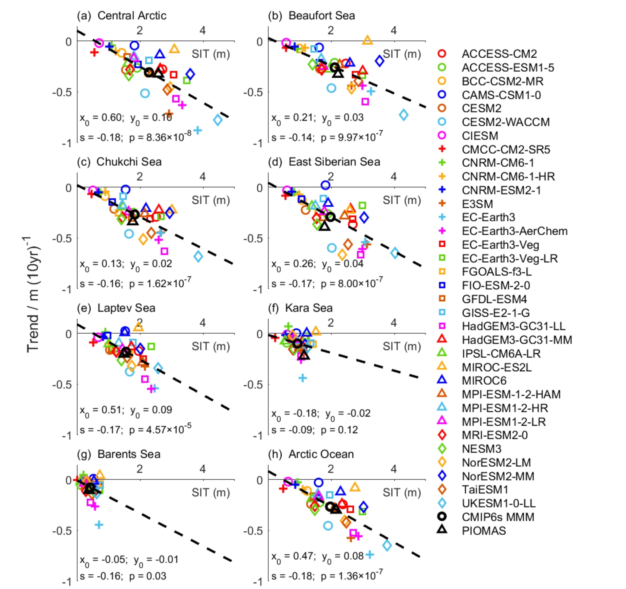
Fig.8.The trend versus the climatological mean of the SIT during 1979–2014 from CMIP6 models and PIOMAS in different seas.x0 and y0 are the X- and Y-axis intercepts, respectively; s is the linear regression coefficient, and p is the confidence level.

The x-intercept, -β0/β, represents the equilibrium SIT(ESIT) when the SIT trend equals zero under the historical forcing, i.e., the minimum SIT under the same historical forcing.The maximum ESIT appears in the Central Arctic Sea and the Laptev Sea, being more than 0.5 m; the minimums,both negative, appear in the Kara Sea and the Barents Sea,which means that these two areas will eventually become ice-free.ESIT for the Arctic Ocean is 0.48 m.

In contrast, the y-intercept, β0, reflects the sea ice recovery potential (RP) when all the Arctic SIT has melted (an ice-free scenario).We suggest that RP reflects the sea ice’s recoverability, which means some processes could enforce the growth of local sea ice and resist the SIT decline caused by global warming.The RP for the Arctic Ocean is about 0.08 m (10 yr)–1.The greatest RP appears in the Central Arctic , being about 0.1 m (10 yr)–1, while the RPs of the Kara and the Barents Seas are both negative.Therefore, the Kara Sea and the Barents Sea most likely meet the ice-free scenario from their ESIT and RP.

Being derived from ensemble models’ results, DR,ESIT, and RP reflect humans’ general understanding of the inherent features of the Arctic sea ice change under the specific radiative forcing.They are insensitive to both the systematic bias of numerical models and the internal climate variability, thus helping assess the features of climate change in different scenarios, especially in future projections.

4.Conclusion and discussion

The simulated Arctic sea ice thickness from 34 CMIP6 models is assessed against PIOMAS data for the period 1979–2014.Most models reasonably produce the spatial pattern of the climatological mean sea ice thickness, although significant inter-model spread exists.Increasing model resolution and properly choosing sea ice model physics can lead to improved SIT simulation.The averaged Arctic SIT of the selected CMIP6 models is about 0.19 m thinner than the PIOMAS data.The most considerable overestimation and underestimation for regional SIT appear in the East Siberian and the Central Arctic, respectively.Most models reproduce a much better sea ice pattern in the growing season than in the melting season.Regardless of the systematic bias, most models can produce the historical SIT declination in each sea and the entire Arctic Ocean.

For the climatological mean and the trend of the Arctic SIT, three indicators, i.e., the decrease ratio (DR), the equilibrium SIT (ESIT), and the recovery potential (RP), are studied.Under the historical radiative forcing, DR is –18%decade–1, ESIT is 0.47 m, and RP is 0.08 m decade–1for the Arctic.Different seas in the Arctic Ocean have similar DRs,ranging from –18% decade–1to –9% decade–1, but their ESITs and RPs vary significantly among models.The Kara Sea and the Barents Sea have the two smallest ESITs and RPs, implying that they are most likely to be ice-free all year round in the future.In contrast, the Laptev Sea and Central Arctic are unlikely to be ice-free.Therefore, DR, ESIT,and RP can reflect the general features of sea ice change from the viewpoint of numerical simulations without knowing the detailed mechanism.

Dynamic and thermodynamic processes modulate sea ice change (Spall, 2019; Yu et al., 2021).Some literature suggests that the thermodynamic processes play a more critical role in the sea ice loss in the whole Arctic Ocean (Bitz and Roe, 2004; Holland et al., 2006; Massonnet et al., 2018), especially in the Chukchi Sea, the East Siberian Sea, and the Kara Sea (Yu et al., 2021).The transpolar drift transports ice dynamically from the Pacific Arctic to the Atlantic Arctic and delivers sea ice out of the Arctic Ocean through the Fram Strait (Ricker et al., 2018; Min et al., 2019).SIT change on a regional scale owns spatial-dependent mechanisms.For example, the SIT change in the central basins is linked to the Atlantic water entering through the Fram Strait(Dörr et al., 2021; Kumar et al., 2021); the SIT in the Laptev Sea is also affected by river runoff (Holland et al.,2006; Park et al., 2020).Moreover, a quantitative analysis to distinguish sea ice’s thermodynamic and dynamic processes is even more complicated and has enormous uncertainties (Spall, 2019; Yu et al., 2021).And the three indicators’regional differences and temporal variations can reflect the competitive relationship among various thermodynamic and dynamic processes in sea ice under a changing external forcing.But this might help us understand the future Arctic climate projections.

Many factors contribute to the biases of model simulation results.Previous studies have shown that the model resolution, sea ice component, and the uncertainty of reference data could have an impact on the biases.Therefore, to improve the results’ reliability, it is necessary to use the data from satellite and in situ observation platforms for further comparison.Moreover, it also should be realized that the evaluation of model simulations should not be limited to the comparison of model simulation results and observation results for a single parameter but should focus on the differences between models and highlight the potential reasons for these differences, which is the next step of this work.

Acknowledgements.This is a contribution to the Year of Polar Prediction (YOPP), a flagship activity of the Polar Prediction Project (PPP), initiated by the World Weather Research Programme(WWRP) of the World Meteorological Organization (WMO).This study was funded by the National Natural Science Foundation of China (Grant Nos.41922044 and 41941009), the National Key R&D Program of China (Grant No.2019YFA0607004 and 2022YFE0106300), the Guangdong Basic and Applied Basic Research Foundation (Grant Nos.2020B1515020025 and 2019A1515110295), and the Norges Forskningsråd (Grant No.328886).