Zhicheng GE, Xuezhu WANG*,3, and Xidong WANG,2

1Key Laboratory of Marine Hazards Forecasting, Ministry of Natural Resources, Hohai University, Nanjing 210098, China

2Southern Marine Science and Engineering Guangdong Laboratory (Zhuhai), Zhuhai 519000, China

3Key Laboratory of Marine Science and Numerical Modeling, Ministry of Natural Resources, Qingdao 266061, China

ABSTRACT This study evaluates the Arctic sea-ice simulation of the SODA3 dataset driven by different atmospheric forcing fields and explores the errors of the Arctic sea-ice simulation caused by the forcing field.We find that the SODA3 data driven by different forcing fields represent a significant systematical error in the simulation of Arctic sea-ice concentration, showing a low concentration of thick ice and a high concentration of thin ice.In terms of sea-ice extent, the SODA3 data from different versions well characterize the interannual variability and declining trend in the observed data, but they overestimate the overall Arctic sea-ice extent, which is related to excessive simulation of ice in the sea-ice margin.Compared to observations, all the chosen SODA3 reanalysis versions driven by different atmospheric forcing generally tend to underestimate the Arctic sea-ice thickness, especially for thick ice in the multi-year sea-ice regions.Inaccurate simulations of Arctic sea-ice transport may partly explain the error in SODA3 sea-ice thickness in multi-year sea-ice areas.The results of different SDOA3 versions differ greatly in the Beaufort Sea, the Fram Strait, and the Central Arctic Sea.The difference in sea-ice thickness among different SODA3 versions is primarily due to the thermodynamic contribution, which may come from the diversity of atmospheric forcing fields.Our work provides a reference for using SODA3 data to study Arctic sea ice.

Key words: Arctic sea-ice, SODA3, simulation and evaluation, sources of model error

1.Introduction

Due to the Arctic's high sensitivity to climate and its important feedback role, it is considered an amplifier and indicator of global climate change (Screen and Simmonds,2010).Furthermore, the spatiotemporal evolution of sea-ice coverage significantly impacts polar marine biogeochemistry, ecosystems, and economics (Kovacs et al., 2011;Smith and Stephenson, 2013; Vancoppenolle et al., 2013).Sea ice has a high albedo, which reflects more solar energy back into space (Maykut, 1982).

The latest Intergovernmental Panel on Climate Change(IPCC, 2022) Special Report on Climate Change and the Ocean and Cryosphere clearly states that: Arctic surface temperatures have tripled in the last two decades, with surface temperatures in the central Arctic higher than in any year since 1900, a change exacerbated by the melting of snow and ice.Sea ice can lead to atmospheric circulation anomalies by affecting local energy balances and through sea-air interactions.Therefore, signals of sea-ice changes can be transmitted from near the polar regions to mid- and high-latitude regions by atmospheric circulation, further affecting midand high-latitude weather and climate (Screen and Simmonds, 2013; Cohen et al., 2014).

The rapid changes in the Arctic climate system have great implications for human survival and development,which affect not only the Arctic land and ocean environment but also the northern hemisphere and global climate.Long time-series sea-ice datasets are required to better understand the changes in sea ice (Guemas et al., 2016).Fortunately,the launch of passive microwave satellites in the late 1960s made it possible to observe Arctic sea ice over large areas for long periods.Due to limitations in the timescale, spatial and temporal resolution, and accuracy of satellite observation data (Laxon et al., 2013), the data do not meet the objectives of all sea-ice research or for scientists seeking to understand the fundamental mechanisms behind sea-ice evolution(Comiso, 2017).Modeling sea-ice data and sea-ice climate models have become effective tools for understanding seaice development and its effects on climate change in this setting (Proshutinsky et al., 2011; Stroeve and Notz, 2015).

However, the variability of real-world sea ice is too complex, and there still exist many uncertainties in model simulations, which primarily include model uncertainties and uncertainties in the atmospheric forcing fields.The Ocean Model Intercomparison Project (OMIP) identifies those improvements that need to be made in models.Two phases of the project are currently underway, the first with 13 models driven by an atmospheric dataset of CORE-II and the second with 11 models driven by an atmospheric dataset of jra55-do.Under the OMIP1 and OMIP2 projects, several studies assessed sea-ice thickness and extent and found that OMIP1 tends to underestimate the declining trends in sea-ice thickness.According to the OMIP2 results, the Arctic sea-ice extent is larger than what is observed in the Greenland-Iceland-Norwegian Seas.Sea-ice concentration in the Northern Hemisphere is underestimated by OMIP1 during summer,while improvements are noted in OMIP2 (Wang et al.,2016; Tsujino et al., 2020).OMIP’s work found that internal variabilities, flaws in the sea-ice model formulations, and the effects of simulated sea-ice on the atmosphere and ocean can all contribute to differences between simulations and observations (Notz et al., 2016).

Sea-ice simulation can be affected by both atmospheric forcing and model uncertainties.Model uncertainty, extensively studied in the OMIPs and by Zheng et al.(2021), also concluded that the uncertainty in the model itself could result in inaccurate sea-ice simulations.However, the effect of different atmospheric forcing fields on sea-ice simulation has been less involved in details.It is essential to investigate the effect of atmospheric forcing fields on model simulations to understand the source of model error.The Simple Ocean Data Assimilation dataset (SODA3, Carton et al., 2018,https://www2.atmos.umd.edu/～ocean/soda3_readme.htm)from the University of Maryland is one of the most extensively used ocean reanalysis datasets.There are five different sea-ice simulation results in the SODA3 dataset, which are forced by the different atmospheric datasets.The SODA3 sea-ice reanalysis product provides an opportunity to evaluate the effect of different atmospheric forcings on sea-ice simulations.To assess the performance of the SODA3 sea-ice simulations, we used an evaluation method similar to that of Zheng et al.(2021).We focus on evaluating the results of representative March and September sea-ice simulations.Afterward, we examine the relationship between sea-ice thickness and atmospheric forcing in greater detail, including dynamic and thermodynamic factors, to investigate the possible effect of atmospheric forcing on March and September sea-ice simulations.

The remainder of this paper is organized as follows.Section 2 describes the data used to validate the SODA3 data set and the method used to diagnose sea ice.In section 3,we evaluate the spatiotemporal variability of sea-ice concentration, thickness, and volume.In section 4, the error of seaice simulations is analyzed in terms of its dynamics and thermodynamics.Section 5 provides a discussion and conclusion.

2.Data and methods

2.1.Data for evaluation

SODA3 reanalysis is produced by simple ocean data assimilation developed by the University of Maryland.SODA3 reanalysis is built on the Modular Ocean Model v5 ocean component of the Geophysical Fluid Dynamics Laboratory CM2.5 coupled model with fully interactive sea ice(Delworth et al., 2012) and an improved horizontal resolution of 0.25° and a vertical resolution of uneven 50 layers (spacing 10 m at boundary layer).The Geophysical Fluid Dynamics Laboratory Sea-ice Simulator used the scheme of dynamics and thermodynamics from Winton (2000) in their sea-ice model.Based on Semtner's three-layer framework, this model replaces the brine content in the upper ice with a variable heat capacity that is more physically realistic.The SODA3 reanalysis product contains several versions forced by different atmospheric datasets.For the convenience of comparison, we chose five sub-datasets among them.A brief introduction of chosen SODA3 dataset is shown in Table 1.

Table 2 displays the observed sea-ice data used for com-parison and evaluation in this study.SODA3 results are compared to satellite observation data of sea-ice concentration based on bootstrap algorithms.The sea-ice concentration data based on a bootstrap algorithm (Comiso., 2017) has been derived using measurements from SMMR, SSM/I, and SSMIS since 1979.Observations of sea-ice thickness were sourced from the joint data merging of CryoSat-2 sea-ice thickness fields, and the thin sea-ice thickness estimates were obtained from the Soil Moisture and Ocean Salinity satellite (Ricker et al., 2017).The time coverage of the seaice thickness data set is from October to April of the following years from 2010.

Table 1.A brief introduction of SODA3 data (DA: Data Assimilation, * Indicates that flux correction has been performed).

Table 2.Data for evaluation.

Sea-ice index products cover the period from 1979 onwards and are comprised of two data sets 1) the near-realtime DMSP SSMIS Daily Polar Gridded Sea-ice Concentrations and 2) the sea-ice concentrations from Nimbus-7 SMMR and DMSP SSM/I-SSMIS Passive Microwave Data.This dataset uses the 15 percent sea-ice concentration contour from satellite observations as a criterion for determining seaice extent because a study of sea-ice concentration at ice edge locations from airborne measurements found that seaice edge best matched the 15 percent sea-ice concentration contour from satellite data (Cavalieri et al., 1991).The monthly average data for sea-ice extent can be computed by summing the daily sea-ice concentration data for each grid cell in a given month, dividing by the total number of days in that month to get the monthly average concentrations for that grid cell, and then deriving the monthly average extent from the 15 percent sea-ice concentration contour.Using this numerical averaging algorithm, this dataset can capture the temporal variation in ice-extent values over a given month.

The latest released Polar Pathfinder Daily 25 km EASEGrid sea-ice drift data from the National Snow and Ice Data Center (Tschudi et al., 2020) are also used to evaluate the SODA3 reanalysis.The melting and freezing seasons data from 1978 to 2020 are included in this observed sea-ice drift dataset, which has been extensively used for modeling and data assimilation.The sea-ice motion data sets are obtained from AVHRR, AMSR-E, SMMR, SSM/I, SSM/I,International Arctic Buoy Program (IABP) buoys, and the National Center for Environmental Prediction (NCEP)/National Center for Atmospheric Research (NCAR) Reanalysis wind data.More details may be found in the user guide(https://nsidc.org/data/NSIDC-0116/versions/4).

The Pan-Arctic Ice Ocean Modeling and Assimilation System (PIOMAS, Zhang and Rothrock, 2003) developed at APL/PSC (Polar Science Center) can simulate the sea-ice volume (Schweiger et al., 2011).This system is a coupled seaice-ocean model with sea-ice concentration (SIC) and SST assimilation using optimal interpolation.Sea-ice concentration data from the NSIDC near-real-time product are assimilated into PIOMAS to improve ice thickness estimates, and SST data from the NCEP/NCAR reanalysis are assimilated in the ice-free areas.Compared to IceBridge, Wang et al.(2016) found that PIOMAS overestimated thick ice around Greenland's north coast and the Canadian Arctic Archipelago (CAA) and underestimated thin ice in the Beaufort Sea.PIOMAS v2.1 is used in this study as reference data for sea-ice volume estimation.

2.2.Methods for evaluation

A numerical method developed by Holland and Kwok(2012) is used to distinguish between changes in sea-ice thickness due to thermodynamic and dynamic processes.It is based on the continuity equation presented by Bitz et al.(2005):

Similar to Holland (2014), we define ∂C/∂tas the ice“intensification” whereCis the sea-ice thickness.The lefthand side of the equation shows the intensification and seaice thickness flux divergence (dynamic), where the flux divergence includes both advection (u·∇C) and divergence(C∇·u).The terms of the right represent the thermodynamic melting/freezing (fc) and mechanical redistribution (r) of ice, which is defined as the residual, mostly determined by heat forcing.Finally, we have four terms in our equation:

Numerous previous studies have used the concentration and thickness tendencies of sea ice to characterize both the thermodynamic and dynamic contributions to sea-ice variability (Holland and Kwok, 2012; Holland and Kimura, 2016;Schroeter et al., 2018; Cai et al., 2020).This method is applied in this study to analyze the SODA3 dataset on the original grid.Sea-ice drift and sea-ice thickness from the SODA3 dataset are chosen to compute the sea-ice thickness tendencies according to Eq.(2).We choose October to February as the freezing season and April to August as the melting season.

3.Difference between SODA3 reanalysis and observation

3.1.Temporal variabilities in the sea-ice extent

In the Arctic, seasonal cycles are one of the most significant features of sea-ice variabilities.Compared with observations, the simulated sea-ice extent from SODA3 characterizes the seasonal cycle well (Fig.1).However, the sea-ice extent is overestimated by SODA3 both in the summer and winter.The discrepancy between the simulated and observed seaice extent peaks in March before gradually decreasing throughout the melting season.SODA3 overestimates the extent of sea ice in winter by 2.5 × 106km2, with little difference between versions from 1979–2015.Compared to winter, the differences in the extent of summer sea ice are more apparent.SODA 3.4.2 has the smallest error, overestimating by approximately 0.4 × 106km2.The largest error is from SODA3.11.2, which overestimates by approximately 2 ×106km2.In summary, the modeling seasonal variation of SODA3 in sea-ice extent over the past 35 years is mostly consistent with the observations.Still, all SODA3 simulations overestimate the extent of sea ice, especially in winter.

To assess SODA3's performance, we compared the annual sea-ice extent between simulations and observations in the months of March and September, which are the representative months of the summer and winter seasons, respectively.At the end of the growing and melting seasons, the extent of sea ice reaches its maximum and minimum in March and September, respectively.Figure 2 shows the temporal evolution of Arctic sea-ice extent in March and September from 1979–2015 for different versions of SODA3 simulations.Although the observed and simulated sea-ice extents differ numerically by a large amount, there is no significant difference between the interannual variability and trends among the different versions of SODA3.The correlation coefficients for March and September are statistically significant at a 99% confidence level, as shown in Table 3.Overall, the sea-ice extent of simulations is highly correlated with observations.SODA3 overestimates the sea-ice extent in March and September from 1981 to 2015, especially in March, contributing to the seasonal cycle pattern in Fig.1.

Data-based trends of March and September sea-ice extent (95% confidence level) are listed in Table 4.Based on Fig.2a, the observed sea-ice extent in March decreased faster than the SODA3 simulation.The rate of decrease in the observations is 0.38 × 106km2yr–1compared to around 0.2 × 106km2yr–1in SODA3.The results for September are more complex, with the observed sea-ice extent decreasing at a rate of 0.88 × 106km2yr–1and SODA3 showing both a faster than observed decrease of 0.91 × 106km2yr–1and a slower decrease of 0.88 × 106km2yr–1.The uncertainty in sea-ice extent interannual variation is greater in summer than in winter, with standard deviations of 0.12 and 0.03 for the rate of decrease in sea-ice extent in summer and winter.

Fig.1.(a)–(e) Seasonal variability of Arctic sea-ice extent from monthly observation data (solid red line) and SODA3(dashed lines) from 1981-2015.The shading indicates ± 2 standard deviations for the observations.(f) The sea-ice extent difference between SODA3 and observations (SODA3 minus observations).

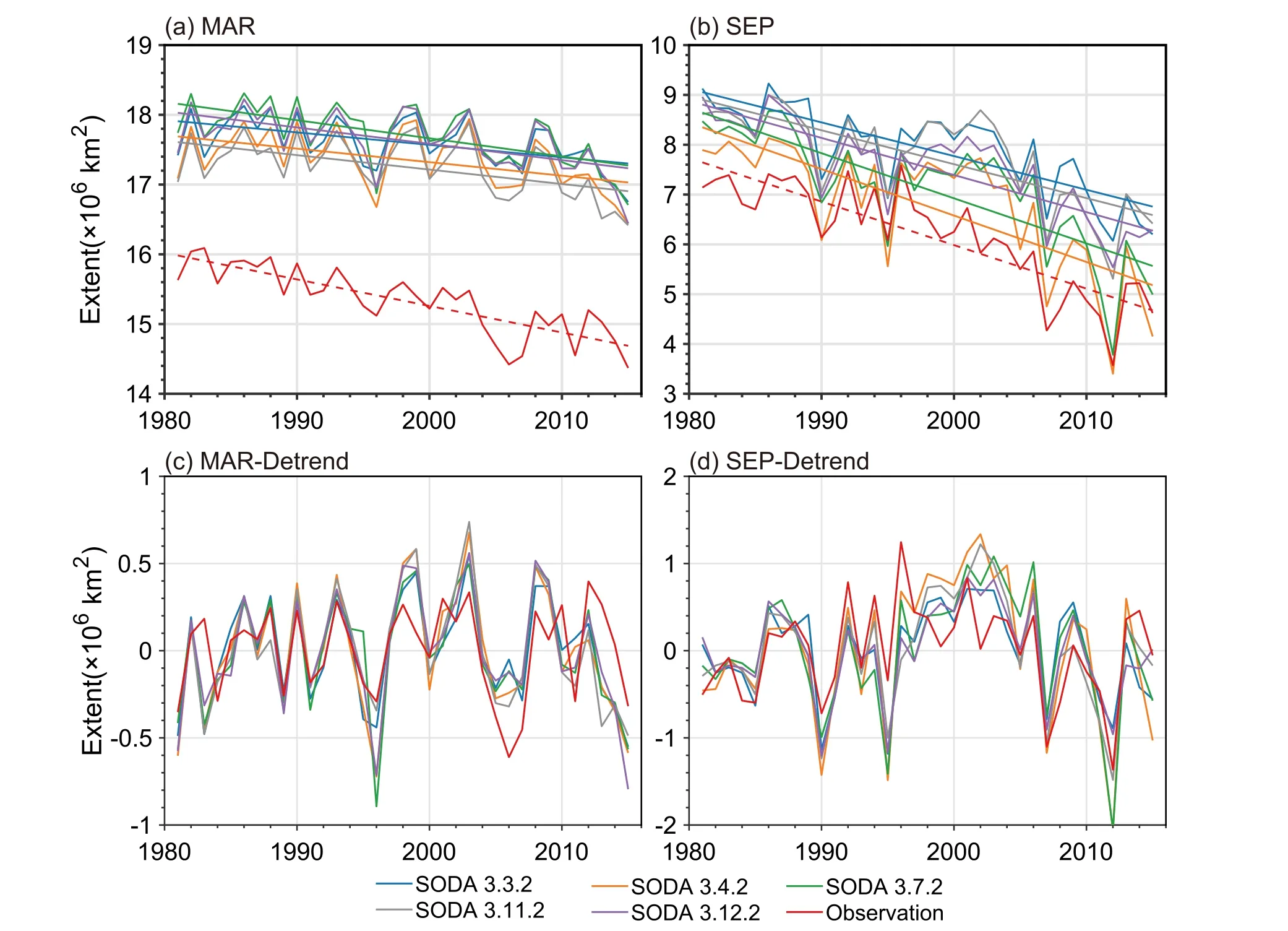
Fig.2.Monthly variability of sea-ice extent for (a) March and (b) September over the period 1981–2015, as well as monthly variability of detrended anomalies of sea-ice extent for (c) March and (d) September.Red solid lines represent observations, and other colored solid lines represent SODA3.

Table 3.The correlation coefficients between SODA3 and observed sea-ice extent from 1981 to 2015.Detrended time series results are shown in brackets (STD: standard deviation).

Table 4.Sea-ice extent trends from 1981 to 2015 at a 95% confidence level (units: 106 km2 yr–1).

Figures 2c and 2d show the temporal variations of the detrended anomalies of the sea-ice extent.From the figures,we can see that SODA3 can well reproduce the interannual variations of sea-ice extent.In March, it is noteworthy that all versions of SODA3 maintained their average correlation coefficients of about 0.68 after the detrending.In September,however, significant differences in the interannual variation of SODA3 after detrending exist among the versions of SODA3.We calculate the correlation coefficients for the time series of sea-ice extent for SODA3 and observation at different periods.In Table 5, the mean correlation coefficient of September sea-ice extent simulated by SODA3 during 1996–2005 is 0.04, significantly lower than the 0.69 and 0.78 that existed during 1981–1995 and 2006–2015, respectively.This phenomenon is not particularly pronounced in the winter months.In some years (e.g., March 2009, March 2006, September 1999, etc.), the observation is increased relative to the previous year, but the results of SODA3 are decreased.The SODA3 dataset's correlation coefficients reveal that the sea-ice extent in September is more difficult to simulate than in March.This phenomenon may be caused by thinner sea ice in September, which is more mobile and thus more sensitive to atmospheric conditions, increasing the difficulty in conducting accurate simulations (Stroeve et al., 2012).

3.2.Spatial distribution of sea-ice concentration

Further, we investigate the error of spatial distribution of the sea-ice concentration in SODA3.Figures 3 and 4 show the spatial distribution of sea-ice concentration in March and September, respectively.The greatest differences between simulated and observed sea-ice concentrations in March are centered in the sea-ice areas of the Fram and Beaufort Straits, particularly in the Fram Strait, which is a major channel for the export of Arctic sea ice.The difference between the different versions of SODA3 in this region,where sea-ice concentrations are close to 100%, is less significant.When sea ice decreases in September, its edge also decreases into the East Elizabeth Sea, Chukchi Sea, Kara Sea, and Barents Sea, and the error of simulated sea ice was significantly higher in these areas.In all simulations, sea-ice concentrations along the sea-ice edge are overestimated,except for SODA3.4.2, where sea-ice concentrations in the interior of the sea-ice edge region are underestimated.SODA3.7.2 has the closest agreement with the observed results among all SODA3 simulations in September.

In addition, the pattern correlation is shown in Fig.5.The pattern correlation is the Pearson product-moment coefficient of linear correlation between two variables at corresponding locations on different maps, which, in this paper,were calculated in the area north of 60°N.The pattern correlation of all SODA3 versions is lower in September than in March, indicating that the spatial distributions of simulations and observations are more inconsistent in September.InFig.5b, the increase in the standard deviation of sea-ice concentration can explain the decrease in pattern correlation between SODA3 and observation.In summer, as sea ice decreases, accurate simulations become more difficult.The Taylor diagram of the sea-ice concentration distribution in the Arctic from SODA3, relative to observations, is shown in Fig.6.Results of satellite observations lie on the positive x-axis, which indicates the reference sea-ice concentration data.There was almost no difference in correlation coefficients for all versions of SODA3 simulations in summer,with a correlation coefficient (root-mean-square difference,RMSD) of 0.92 (0.15).In winter, SODA 3.3.2 and SODA 3.11.2 have similar results, with a correlation coefficient(root-mean-square difference, RMSD) of 0.94 (0.23).SODA3.4.2 yields a correlation coefficient of 0.95 and an RMSD of 0.21, while SODA3.7.2 produces values of 0.95 with 0.22, respectively.

Table 5.The correlation coefficient between the simulation results of SODA3 in September and the observed data over different periods(March correlation coefficient in parentheses).

Fig.3.Climatology distribution of March sea-ice concentration (1981–2015).(a) Observations and (b–f) differences in simulations relative to observations.The Magenta line represents the 15% sea-ice concentration contour in the observed data.

Fig.4.Same as in Fig.3, but for September.

Fig.5.The evolution of the pattern correlation of sea-ice concentration between the SODA3 and the observations in(a) March and (b) September from 1981–2015.The magenta points in (b) indicate the standard deviation for each period of five years.The figure also shows the interannual trend of standard deviation.

Fig.6.Taylor diagram comparing simulation results of sea-ice concentration in different versions of SODA3 and observation for (left) March and (right) September.

3.3.Evaluation of sea-ice thickness

When used as an indicator for evaluating sea-ice simulation results, the sea-ice concentration does not fully reflect the SODA3 capabilities.Although the value of sea-ice concentration ceases to increase when sea-ice concentration reaches 1, the sea-ice thickness continues to increase.Compared to sea-ice concentration, sea-ice thickness is a better indicator of how dynamics and thermodynamics affect sea ice.Therefore, it is essential to assess the performance of SODA3 sea-ice thickness.In the Arctic, measurements of the sea-ice thickness are discontinuous over time due to the polar nights.Therefore, the sea-ice thickness should be evaluated within the time period covered by the available observations (Tilling et al., 2015).

To better understand the difference between the SODA3 sea-ice thickness and the observed data, we calculate the proportion distribution of the average sea-ice thickness from October to April based on the observed (Cryosat-SMOS) and SODA3 data, as shown in Fig.7.Observations and SODA3 demonstrate good agreement between the proportion distribution of sea-ice thickness less than 0.5 m, indicating SODA3's good capability in simulating sea-ice with thickness less than 0.5 m.Within the interval between 0.5 and 1.1 m, SODA3 overestimates the proportion of sea-ice thickness.However, when the sea-ice thickness exceeds 1.5 m,the results are reversed, and the proportion of SODA3 in this interval is significantly lower than observed.These results indicate that SODA3 may be incapable of modeling thick ice effectively.

To better assess the spatial distribution of Arctic sea-ice thickness, the spatial distributions of SODA3 and observed sea-ice thickness, and the differences between them are shown in Fig.8.The observed data of sea-ice thickness during 2011 to 2015 come from the product of CryoSat2-SMOS.SODA3 data is interpolated into the CryoSat2-SMOS grid to directly compare with observed data.We use the October to April average directly for comparison because of the unavailability of the Arctic sea-ice observations.The patterns of SODA3 and observed results are generally consistent,and the differences among SODA versions are small.The Arctic sea ice is divided into two groups by the CryoSat2-SMOS dataset: first-year ice and multi-year ice.First-year ice is thicker than 30 centimeters but has not survived a summer melting season.Multi-year ice describes ice that has survived a summer melting season and is much thicker than younger ice, typically ranging from 2 to 4 meters thick.The sea-ice survival zone is defined as the area in the grid point where multi-year ice occurs more than 50%.By comparing the edge line of this zone, we can see that the discrepancy between simulations and observations is concentrated in the northern parts of the Canadian Archipelago and Greenland,as well as the Fram Strait, which is the Arctic sea-ice survival zone.In all versions of SODA3, SODA3.4.2 shows the greatest difference from observations, while the other versions have approximately the same differences.

Fig.7.Proportion distribution of mean sea-ice thickness from October to April, over 2011–2015.The red line is the result of Cryosat-SMOS, and other lines indicate the result of SODA3.

In addition, Fig.8g shows the frequency distribution of the sea-ice thickness difference between SODA3 and the observed, which mostly ranges from –1 to 0.5 m, accounting for almost half of all thickness differences.For each 25-km ICE-Sat grid cell, Kwok et al.(2009) estimated that the uncertainty of ice thickness is about 0.5 m.From the results of the sea-ice thickness assessment, nearly 50% of the area in SODA3 has errors outside the observed range.Compared with the simulation of sea-ice concentration, the SODA3 simulation of sea-ice thickness has a larger bias.Finally, Fig.9 is a Taylor diagram of the sea-ice thickness distribution in the Arctic from SODA3 relative to observations.The results of Crysat2-SMOS lie on the positive x-axis, which indicates the reference sea-ice thickness data.SODA3.3.2 and SODA3.4.2 have a lower correlation coefficient (0.88) and RMSD (0.22 m), which is due to the underestimation of seaice thickness in thick ice regions.Other SODA3 simulations showed almost identical correlation coefficients and RMSD values of 0.89 and 0.21 m, respectively.

Operation IceBridge data (Sato and Inoue, 2018) are only available in March and April of a given year.Although each observation lasts only a few hours, it covers a large area in the western Arctic.These data allowed us to further evaluate the performance of the SODA3 sea-ice thickness in the western Arctic.The scatter plot of sea-ice thickness reveals a significant correlation between SODA3 and in-situ observations during spring (with an average thickness of 0.7 m), with a mean discrepancy of –0.88 m (Figs.10b–f).The majority of scatter points in all SODA3 simulation results fall below the diagonal of the coordinate system, meaning that simulated sea-ice thickness is thin.Figure 10a shows that most observation stations are in multi-year ice zones.The high RMSD of SODA3 results indicates that the model has high uncertainty in reproducing the thick ice in the multi-year ice zones.Figure 10 also shows that the bias is largest in SODA3.4.2 and lowest in SODA3.12.2 among all SODA3 versions compared with CryoSat2-SMOS satellite observations and IceBridge in-situ observations.

Sea-ice volume comparisons can provide a comprehensive assessment of sea-ice concentration and thickness.The product of the sea-ice thickness at each grid cell of the data,the sea-ice concentration, and the corresponding grid area is used to determine the monthly Arctic sea-ice volume.The time series of observed sea-ice growth periods (October to April) and SODA3’s sea-ice volumes are shown in Fig.11,along with errors in the inversion algorithm based on the observed data from 2011 to 2015.The results show that all versions of SODA3 capture the significant seasonal cycle in the observed volume of Arctic sea ice.However, SODA 3.3.2 tends to underestimate sea-ice volume in winter, and SODA 3.4.2 tends to underestimate sea-ice volume in summer, while the sea-ice volumes from the other three versions of SODA generally are within the error of observations.In Fig.11, PIOMAS, one of the most often used datasets for Arctic research, is compared against SODA3.PIOMAS has a similar sea-ice volume to SODA3 in summer but exceeds all versions of SODA3 in winter.This phenomenon is mainly due to excessively fast sea-ice growth during the freezing period,which is also concluded by Wang et al.(2016).

4.Possible error sources of SODA3 sea-ice thickness

It is more important to explore the reasons for the difference between simulated and observed sea-ice thickness, compared with any other sea-ice property, since the sea-ice thickness is a more integrated indicator of changes in sea-ice than sea-ice concentration.Many factors contribute to the discrepancy between simulations and observations concerning sea-ice evolution, such as uncertainties in both the SODA3 and observation.According to Zheng and Zhu (2008), the primary sources of model errors include flaws in the parameterization of physical processes, boundary condition errors, and numerical solution errors.In the next subsection, we discuss the sources of sea-ice thickness error of SODA3 and the difference among different versions of SODA3 to improve the model's performance for simulating sea ice.

Fig.8.Difference of sea-ice thickness between SODA3 and observation from October to April during 2011–2015.(a)–(f)Spatial distribution.The areas surrounded by the magenta line indicate the multi-year sea-ice zone.Panel (g) illustrates the fractional distribution of the sea-ice thickness difference.

Fig.9.Taylor diagram comparing simulation results of the seaice thickness (Oct–Apr) in different versions of SODA3 and observation.

4.1.Sources of sea-ice thickness error of SODA3

The wind causes ridging and rafting of ice by driving the ocean's surface circulation and sea-ice transport.Serreze and Barry (1988) estimate that the geostrophic wind played a significant role in sea-ice drift in the Arctic Ocean.Figures 12a and 12b depict the geographical distribution of Arctic sea-ice drift from CryoSat2-SMOS data.The magenta line represents the boundary line between multi-year and oneyear sea ice from CryoSat2-SMOS data.The interpolated SODA's sea-ice drift data and NSIDC's sea-ice drift data onto the boundary line are presented in Figs.12c and 12d.

Fig.10.(a) Locations of IceBridge measuring sea-ice thickness from 2009 to 2014, and (b–f) scatterplot between sea-ice thickness from SODA3 (y-axis) and sea-ice thickness from Operation IceBridge (x-axis).

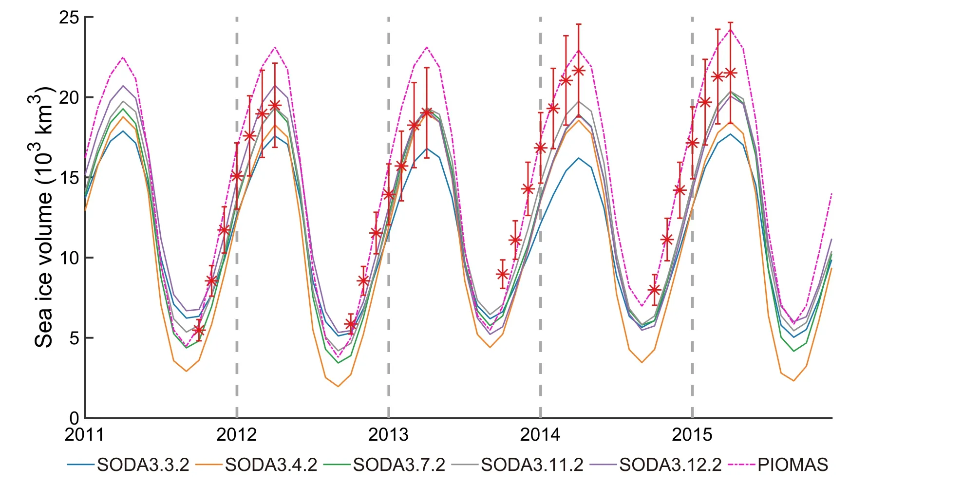
Fig.11.The Arctic sea-ice volume from SODA3 and PIOMAS (magenta dashed line) over 2011-2015.The red points and red error bars indicate Cryosat-SMOS monthly sea-ice volume and sea-ice volume uncertainty,respectively.

Figure 12a shows that in March, the export of sea ice from the multi-year sea-ice area mainly appears in the Greenland and Beaufort Seas, while input occurs in the central Arctic.Figure 12c shows the sea-ice drift velocity perpendicular to the multi-year sea-ice line in Fig.12a.Positive values indicate sea-ice movement toward the multi-year sea-ice zone,and negative values indicate movement outward.SODA3 simulates average drift velocities of sea ice as 0.17 m s–1in the Greenland Sea and 0.01 m s–1in the Beaufort Sea,which are much higher than observed drift velocities of 0.087 m s–1and 0.004 m s–1.Thus, the Canadian Archipelago and northern Greenland accumulate less sea ice, resulting in a thinner sea-ice thickness simulation in Fig.12 compared to observations.In September, the simulated sea-ice drift velocities by SODA3 in the Greenland Sea and Beaufort Sea are 0.06 m s–1and 0.03 m s–1, respectively, compared to the observed drift velocity of 0.03 m s–1, which may result in a difference between SODA3 and observed sea-ice thickness in Fig.12.Despite SODA3 is driven by different atmospheric forcing fields, the simulations of sea-ice drift are nearly identical across versions.These results mean that the SODA3 simulations tend to overestimate the drift speed of sea ice.

4.2.Sources of sea-ice thickness discrepancies among SODA3 versions

To further explore the differences in sea-ice thickness simulations among SODA datasets, Figs.13 and 14 present the Arctic sea-ice thickness budget.Its intensification∂C/∂tis shown in the first row, equivalent to the sum of the other two rows.The Arctic sea-ice thickness budget calculated using SODA3 is consistent with the model ice volume budget of Bitz et al.(2005) and Lindsay and Zhang (2005), which shows that dynamic ice fluxes cause sea-ice to freeze near coastlines and melt at unbounded ice edges.

In general, the results of all versions of SODA3 show little difference during the freezing season.We begin by comparing the differences among the different versions of SODA3 in terms of intensification.Compared with the member mean of SODA3, SODA3.4.2 exhibits the fastest sea-ice growth rate, and SODA3.3.2 exhibits the slowest sea-ice growth rate, while other SODA3 versions show negligible differences from the member mean.The effect of dynamics is to decrease sea-ice thickness in the central Arctic and increase sea-ice thickness at the margins.Compared to the member mean of SODA3, differences in the dynamic contribution of the SODA3 simulation results are mainly in the Fram Strait and the Bering Strait, with such differences being particularly pronounced in the Fram Strait.It is also noteworthy that the dynamic contribution of SODA3.4.2 is stronger in the center of the Arctic than in other versions of SODA3.The root-mean-square error for all the SODA3 simulations in the freezing season is the lowest for SODA3.7.2,SODA3.11.2, and SODA3.12.2.The second-lowest rootmean-square error is for SODA3.3.2, and the highest is for SODA3.4.2.

Similar to the freezing season, SODA3.4.2 showed a faster rate of sea-ice melt during the melting season,whereas SODA3.3.2 showed a slower rate of melt during the freezing season.The dynamic contribution shows only slight differences in the Fram Strait.Based on the rootmean-square error (RMSE), SODA 3.3.2 and SODA 3.4.2 significantly differ from the other versions, especially in summer.The spatial distribution of thermodynamic is almost the same as the residual, while the impact of dynamics on the spatial distribution of the residual can be neglected.Thus, the residual term is primarily responsible for the discrepancy in the SODA3 Arctic sea-ice thickness simulations.

5.Summary and discussion

Fig.12.NSIDC observations of sea-ice drift averaged over (a) March and (b) September of 1981 to 2015.The magenta line in (a) and (b) is the dividing line between multi-year and one-year sea ice.Panels (c) and (d) depict seaice drift velocities perpendicular to the magenta line, and positive numbers indicate that sea ice has moved into the region.Units are m s-1.

Since the early 1970s, the Arctic Ocean has lost over 40% of its summer sea-ice cover.Climate change has resulted in dramatic changes in Arctic sea ice.Thus, the quality of Arctic sea-ice data has received increasing attention.The evaluation of the sea-ice model and modeling data is important for improving the sea-ice model.In this study,five different versions of the SODA3 dataset over the period 1981–2015 are analyzed to assess the spatial and temporal variability and trends in Arctic sea ice.The SODA3 dataset characterizes a reasonable seasonal variation pattern as well as a decreasing trend of sea-ice extent, with small differences among different versions.However, the sea-ice extent of SODA3 is much higher than the observations.The underestimated concentration in the sea-ice edge zone by SODA3 is responsible for the inaccurate sea-ice extent.Moreover,SODA3 and observations only show different spatial distributions of sea-ice concentration in the ice edge region in March and September, with fewer discrepancies in March and larger differences in September.

Additionally, SODA3 underestimates the thickness of sea ice, especially in areas with multi-year sea ice.Sea-ice drift analysis shows that a high sea-ice drift rate of SODA3 results in more sea-ice transport from the multi-year sea-ice area to lower latitudes, which causes thinner sea-ice thickness simulations.Although the atmospheric forcing driving the different versions of SODA3 differs, the differences in the distribution among them compared to observations is consistent,implying that the uncertainty of the model itself is mainly responsible for the inaccurate sea-ice thickness simulations.

Further calculations of the sea-ice thickness budget are made to investigate the effects of dynamics and thermodynamics on sea-ice thickness among the different versions of SODA3.The thermodynamic contribution can be explained by residuals in the sea-ice thickness budget (Holland and Kimura, 2016).Among the different versions of SODA3,the differences in sea-ice thickness are mainly due to thermodynamics.The impact of dynamics is significant only in parts of the Arctic, which is not enough to affect the overall Arctic sea ice on a monthly timescale.

Fig.13.Sea-ice thickness budget components of the freezing season (Oct–Feb), including (from top to bottom) the intensification, dynamic, and residual terms.The first column (from top to bottom) selects the member mean of five versions as the reference group, while the last five columns show the differences between the member mean of SODA3 and the other versions.Units are cm (5 d)–1.The figure indicates the root-mean-square error (RMSE) of the simulation results and the reference group in the upper-left corner.

Fig.14.Same as in Fig.13, but for the melting season (Apr–Aug).

The sea-ice dynamic and thermodynamic processes are important in determining thickness changes.In the SODA reanalysis system, atmospheric forcings contribute differently to both sea-ice processes, leading to differences in simulated sea-ice thickness.The dynamic contribution of SODA3 forced by different atmospheres is similar, and simulated sea-ice drift is higher than in observations.Thus, overestimating sea-ice drift is a systematic error in the SODA reanalysis system.In the melting and freezing seasons, the thermal contribution is lower than the member mean in SODA3.3.2,and its sea-ice thickness is the thinnest compared to the others.This implies that MERRA2 negatively affects the simulation of SODA3.3.2 in terms of sea-ice thickness.The results of SODA3.4.2 forced by ERA-I are opposite to SODA3.3.2.During the melting and freezing seasons, the thermal contribution is higher than the member mean, resulting in thinner sea-ice thickness simulations than the other versions.In other words, ERA-I also negatively impacts the simulation of sea-ice thickness.In addition, other three versions of SODA3, SODA3.7.2, SODA3.11.2, and SODA3.12.2, are forced by JRA-55, DFS5.2, and JRA55-DO, respectively.There are slight differences between them in terms of their dynamic and thermal contributions during the melting and freezing seasons, which also leads to similarities in their seaice thickness simulation results.

To calculate the thermodynamic contribution, the dynamic contribution is subtracted from the intensification rate of sea ice.The usefulness of such a calculation method has some limitations; the residual term includes not only the thermodynamic contribution but also the mechanical redistribution terms associated with ridging and rafting.Therefore,it is inaccurate to treat the residual solely as a thermodynamic component when discussing the overall thermodynamic contributions to sea ice.A future study could use the output from the online model to investigate the thermodynamic and dynamic contributions associated with the atmospheric forcing of Arctic sea ice.

Acknowledgements.The authors are grateful to the providers of the publicly accessible data used in the paper.This study is supported by the Opening Project of Key Laboratory of Marine Science and Numerical Modeling, MNR (2020-ZD-01),the Special Funds for Creative Research (2022C61540), the National Natural Science Foundation (Grant Nos.41776004,41876224), the Fundamental Research Funds for the Central Universities (B210203020), and the Opening Project of Key Laboratory of Marine Environmental Information Technology (20195052912).