Liang ZHAO, Yunwen LIU, Yihui DING, Qingquan LI, Wei DONG, Xinyong SHEN,Wei CHENG, Haoxin YAO, and Ziniu XIAO*

1State Key Laboratory of Numerical Modeling for Atmosphere Sciences and Geophysical Fluid Dynamics (LASG),Institute of Atmospheric Physics, Chinese Academy of Sciences, Beijing 100029, China

2Key Laboratory of Meteorological Disaster, Ministry of Education/Joint International Research Laboratory of Climate and Environment Change/Collaborative Innovation Center on Forecast and Evaluation of Meteorological Disasters,Nanjing University of Information Science and Technology, Nanjing 210044, China

3Neijiang Meteorological Bureau, Neijiang 641000, China

4China Meteorological Administration, National Climate Center, Beijing 100081, China

5Key Laboratory of Geoscience Big Data and Deep Resource of Zhejiang Province, School of Earth Sciences,Zhejiang University, Hangzhou 310058, China

6Southern Marine Science and Engineering Guangdong Laboratory (Zhuhai), Zhuhai 519082, China

7Beijing Institute of the Applied Meteorology, Beijing 100029, China

ABSTRACT An enhanced Warm Arctic–Cold Eurasia (WACE) pattern has been a notable feature in recent winters of the Northern Hemisphere.However, divergent results between model and observational studies of the WACE still remain.This study evaluates the performance of 39 climate models participating in the Coupled Model Intercomparison Project Phase 6(CMIP6) in simulating the WACE pattern in winter of 1980–2014 and explores the key factors causing the differences in the simulation capability among the models.The results show that the multimodel ensemble (MME) can better simulate the spatial distribution of the WACE pattern than most single models.Models that can/cannot simulate both the climatology and the standard deviation of the Eurasian winter surface air temperature well, especially the latter, usually can/cannot simulate the WACE pattern well.This mainly results from the different abilities of the models to simulate the range and intensity of the warm anomaly in the Barents Sea–Kara seas (BKS) region.Further analysis shows that a good performance of the models in the BKS area is usually related to their ability to simulate location and persistence of Ural blocking (UB),which can transport heat to the BKS region, causing the warm Arctic, and strengthen the westerly trough downstream,cooling central Eurasia.Therefore, simulation of UB is key and significantly affects the model’s performance in simulating the WACE.

Key words: warm Arctic–cold Eurasia pattern, Arctic amplification, CMIP6, simulation evaluation, extreme climate,blocking highs

1.Introduction

The rate of warming in the Arctic region was almost twice the global average during recent decades, and there is high confidence that this trend will continue (IPCC, 2021).This phenomenon is referred to as Arctic amplification (Serreze and Francis, 2006).At the same time, the frequency and intensity of extreme events in the midlatitudes of Eurasia, especially persistent low-temperature events in winter,are reported to be increasing (Cohen et al., 2014; Johnson et al., 2018).The warming Arctic accompanied by frequent cold events in Eurasia is reflected in the second mode of the empirical orthogonal function (EOF2) of the Eurasian winter surface air temperature (SAT) and is defined as the Warm Arctic–Cold Eurasia (WACE) pattern (Overland et al.,2011; Cohen et al., 2012; Inoue et al., 2012; Mori et al.,2014).Moreover, the weight of this temperature mode has strengthened since 1998 (Jin et al., 2020).

Previous studies have indicated that the WACE pattern is related to the change of Ural blocking (UB) (Luo et al.,2016a, b; Yao et al., 2017; Jin et al., 2020; Ye and Messori,2020; Kim et al., 2021; Luo et al., 2022; Zhao et al., 2022)and decrease in sea ice concentration (SIC), especially in the Barents Sea–Kara seas (BKS) region (e.g., Cohen et al.,2012, 2014; Mori et al., 2014; Screen et al., 2014; Wegmann et al., 2018).Eurasian cold anomalies were found to be dependent on the weak strength and vertical shear of the mean westerly wind over mid–high-latitude Eurasia, which induce a slow growth of blocking (Yao et al., 2017; Luo et al., 2018;Ye and Messori, 2020).The weak westerly wind is associated with a warm Arctic by changing the meridional temperature gradient.And Arctic warming can increase the persistence of UB through reducing the background meridional potential vorticity gradient (Luo et al., 2019).Thus, the variability of UB is usually crucial for the variation of the WACE pattern.A recent study shows that high-latitude blockings over the north of the Ural Mountains and the North Pacific extending into the Arctic region can be more related to the WACE pattern than the Arctic oscillation (Zhao et al., 2022).The concurrent blockings induce a warmer Arctic by simultaneously transporting large amounts of moisture and heat.Therefore,the simulation of blocking, especially in the Ural and BKS regions, is likely a key to performance in simulating the WACE pattern.

The simulation capability for the WACE pattern is an important prerequisite to revealing the causes of climate change in winter and extreme events in the Northern Hemisphere.Although studies have shown that most models participating in the fifth phase of the Coupled Model Intercomparison Project (CMIP5) (Taylor et al., 2012; Cohen et al., 2020)can simulate the trend, climatology, and first mode of Eurasian SAT, these models tend to overestimate (underestimate) the winter SAT in central (northern) Eurasia or have a southward shift in Arctic warming (Miao et al., 2014; Zhou et al., 2014; Chen et al., 2019; Cohen et al., 2020; Wang et al., 2020).This leads to a much weaker WACE pattern than the actual one.Most CMIP5 models cannot simulate the magnitude of SIC decrease and the cloud variability in the Arctic well (Boeke and Taylor, 2018; Wang et al., 2020), and no strong response of the midlatitude atmosphere to the SIC is found in some climate models (Liang et al., 2020; Warner et al., 2020).In fact, a response of cyclonic or anticyclonic circulation is likely non-linear in relation to the magnitude of sea ice loss (Petoukhov and Semenov, 2010; Yang and Christinsen, 2012; Semenov and Latif, 2015).So, the physical mechanisms of the WACE pattern revealed by the CMIP5 models may not be sufficiently convincing.

At present, in the sixth phase of CMIP (CMIP6; Eyring et al., 2016), the WACE pattern still frequently appears in recent winter temperatures.Compared with the CMIP5 models, some progress has been reported in the CMIP6 models–for example, the spatial resolution and the parameterization of cloud microphysical processes in the Earth system(such as biogeochemical cycles and ice sheets) (Eyring et al.,2019).Furthermore, the CMIP6 models were reported to be able to simulate a stronger warming trend than the CMIP5 models, and the results are closer to the observations (Nie et al., 2019).Additionally, the simulation of SAT in China by the CMIP6 models shows a smaller cold deviation (Jiang et al., 2020).The CMIP6 models perform better in the simulation of global extreme climate events and their trends, especially in the high latitudes of the Northern Hemisphere(Chen et al., 2020).

Although these evaluation studies have partially shown that the simulation results of the CMIP6 models have improved in terms of the global or local SAT (Parsons et al.,2020), there are still few evaluations of the CMIP6 models for the Eurasian winter WACE mode.Whether the current CMIP6 models have sufficient simulation ability for the WACE mode and corresponding atmospheric circulation pattern in the key regions is still unknown.We therefore evaluated the ability of the CMIP6 models to simulate the winter SAT and the leading modes, especially the WACE pattern,and analyzed the reasons for the differences in the simulation results in key regions.

2.Data and methods

2.1.Data

The monthly mean 2-m temperature and 500-hPa geopotential height (Z500) were obtained from the European Centre for Medium-range Weather Forecasts ERA5 reanalysis dataset with a horizontal resolution of (0.25° × 0.25°), available from 1979 to the present day (Hersbach, 2020; https://cds.climate.copernicus.eu/).SIC data were obtained from the Met Office Hadley Centre (Rayner et al., 2003; https://www.metoffice.gov.uk/hadobs/hadisst/).We used the outputs of 39 models from CMIP6 Historical, whose variant label was r1i1p1f1 and historical simulation had been completed (Eyring et al., 2016; https://esgf-node.llnl.gov/projects/cmip6/).The monthly mean 2-m temperature, Z500,and SIC data in simulations were used.In addition, we also used a number of models that provided daily data of Z500(including CanESM5, CESM2, CESM2-FV2, CESM2-WACCM, EC-Earth3, EC-Earth3-Veg-LR, IPSL-CM6ALR, MIROC-ES2, MPI-ESM-1-2-HAM, MPI-ESM1-2-LR,and NorCPM1) and 2-m temperature (including CanESM5,CEMS2, CESM2, EC-Earth3, INM-CM5-0, IPSL-CM6ALR, and MPI-ESM-1-2-HAM).The historical experiment is a simulation of the historical climate with a time period of 1850–2014; the piControl experiment maintains the external forcing at the level of 1850.Table 1 presents a brief description of these CMIP6 models, including the model names,country of origin, their horizonal resolution, and number of levels of the atmospheric components.The daily 500-hPa geopotential height data and 2-m temperature was taken from NCEP/NCAR on a 2.5°×2.5° grid (Kalnay et al., 1996;https://psl.noaa.gov/).For convenience, the time period from 1979 to 2014 of the historical experiments was used for comparison with the observations, and both the models and the observational data were remapped onto the same(1° × 1°) grid.

2.2.Methods

In this study, winter is defined as January and February of the current year and December of the previous year.The multimodel ensemble (MME) is calculated by averaging the variables over all the models with equal weighting.The S index provided by Taylor (2001), which combines the ratioof spatial correlation coefficient (R) and standard deviation(^σf) between the model and observation, is used to quantitatively evaluate the simulation ability of the model.TheR0is the maximum correlation coefficient of the 39 models.The S index is between 0 and 1; the closer to 1, the better the simulation effect (Taylor, 2001; Hirota et al., 2011).The index is defined as:

Table 1.Information about the CMIP6 models used in this study.

The one-dimensional blocking index created by Tibaldi and Monlteni (1990) (TM) is used to identify the blocking events.The TM index uses the reversal of the longitude gradient of the 500-hPa potential height field to detect blocking high pressure.This method can be used to intuitively understand the frequency of blocking high at each point in the two-dimensional plane.GHGS and GHGN are calculated at three latitudes: ϕ0= 60°N+ ∆ , ϕn= 80°N+ ∆ , and ϕs= 40°N+∆ , where ∆=–5°, 0°, and 5° of latitude.When GHGS>0 and GHGN<–10 gpm(°lat)–1for any one of the three values of ∆,a blocking can be considered to have occurred.

3.Climatology and standard deviation of the winter SAT in Eurasia

We evaluated the simulations of the climatology and standard deviation of the winter SAT in Eurasia by the CMIP6 models.For the climatology, the observational results show a northward decrease in the mean SAT in the Eurasian winter.There is a low-temperature center in northeast Asia, and the distribution of the 0°C line almost coincides with the coastline in the area north of 40°N (Fig.1a).The MME can simulate the characteristics of the spatial distribution(Fig.1b).However, the difference field (Fig.1c) shows that,in general, the MME underestimates the actual SAT.In the BKS region, the model underestimates the SAT by at least 7°C compared with the observational results.In addition,there are clear overestimations in northeast Asia and large deviations on the Tibetan Plateau.

Fig.1.Climatological SAT (shading; units: °C) in winter for (a) the ERA5 dataset, (b) the MME, and (c) the difference (shading; units: °C) between the MME and the ERA5 dataset in Eurasia (20°–90°N, 0°–180°E).Standard deviation of the SAT (shading; units: °C) in winter for (d) the ERA5 dataset, (e) the MME, and (f) the difference(shading; units: °C) between the MME and the ERA5 dataset in the same area.The green box indicates the BKS region.

The observational results show that there is a large standard deviation, which can reach 5°C, in the BKS region.There is also an area with a large standard deviation on the Eurasian continent in northern Eurasia (near the Ural Mountains) (Fig.1d).The spatial distribution of the MME is consistent with the observations, indicating that the models can roughly simulate the main temporal characteristics of the winter SAT in Eurasia (Fig.1e).However, the areas with large deviations between the models and observations are mainly located in the BKS region, the Norwegian Sea on the northern side of Eurasia, and the Sea of Okhotsk on the eastern side of Asia (Fig.1f).Between the north and south of the Barents Sea, a dipole of deviations exists.These areas are more affected by high-latitude blocking and sea ice.This result shows that the models’ ability to simulate changes in the SAT in the Arctic region is weaker than that at midlatitudes,suggesting that this simulation ability may be related to the model’s ability to simulate the sea–air system in these regions (e.g., blocking highs and sea ice).

Figure 1 assesses the ability of the MME to simulate the climatology and standard deviation of the winter SAT in Eurasia (20°–90°N, 0°–180°E).We used Taylor diagrams to evaluate the performance of 39 models (Fig.2).The models produced a good overall simulation of the spatial distribution of the climatology, and the spatial correlation coefficients(SCCs) were all >0.94 (Fig.2a).The normalized standard deviation was mostly >1.This shows that all the models–except E3SM-1-0, E3SM-1-1, E3SM-1-1-ECA,and MRI-ESM2-0–overestimate the spatial standard deviation of the SAT.In general, except for the large error between FGOALS-g3, CAS-ESM2-0, GISS-E2-1-G-CC,and BCC-ESM1 and the observations, the other models perform well (Fig.2a).There are large inter-model spreads among the models for the standard deviation (Fig.2b).The SCC between the models and the observations is roughly between 0.6 and 0.9, and only the result of the MME is>0.95.Unlike the climatology, the normalized standard deviation is mostly <1.In general, CanESM5, CESM2, E3SM-1-1, E3SM-1-1-ECA, and HadGEM3-GC31-MM perform better in simulating the standard deviation.

4.Dominant modes of the winter SAT in Eurasia

We evaluated the CMIP6 simulation of the main modes of the winter SAT in Eurasia.Figure 3 shows the EOF results for the ERA5 data and the MME for the winter SAT in Eurasia (20°–90°N, 0°–180°E).In the observations,EOF1 represents overall warming (Fig.3a) and EOF2 represents the WACE pattern of a warmer Arctic and colder Eurasia(Fig.3b).And it can be clearly seen that the WACE pattern is linked to height anomalies over the UB region and the BKS region.The EOF2 mode likely reflects the WACE pattern associated with the UB.By combining these results with the evolution of the normalized principal components,we found that PC1 is mainly characterized by interannual changes (Fig.3c).PC2 changes from a negative phase to a positive phase around 2005 and has clear interdecadal characteristics (Fig.3d).We therefore defined PC2 as a time series characterizing the WACE pattern.

We performed EOF analysis on the winter SAT of each model in CMIP6 and then found the ensemble average to obtain the MME of the EOF.Spatially, the MME can simulate the uniform warming in EOF1 (Fig.3e).And the EOF2 mode of the MME SAT (Fig.3f), similar to observation(Fig.3b), can represent the WACE pattern.However, interdecadal change of Z500 in CMIP6 is seriously overestimated and has some zonal and meridional shift, although a high center of Z500 anomaly exists in 20°–60°E close to observation.The interdecadal variation of PC2 can also be roughly simulated, with the phase transition around 2003 (Fig.3h),which is close to the observational results around 2004(Fig.3d).The deviation likely results from the simulation errors of interannual-scale changes of CMIP6 models.Yearto-year variability will mainly differ in the simulations as the forcing mainly involves slow trends (apart from volcanic episodes).The PC2 of the MME (the average of the individual PC2s) lies between –0.4 and 0.4, which is significantly smaller than the observation.This is because the set of multiple modes has an offset on average.In a single model, there are problems such as the insignificant interdecadal variation trend, the early and late mutation years, and the opposite direction of the phase transition from the observations, which make the ensemble-averaged coefficients decrease significantly and show only weak variation characteristics (Fig.S1 in the Electronic Supplementary Materials, ESM).

From the perspective of the variance contribution rate,the 29.50% of the variance explained by the first EOF mode of the MME is fairly close to the observed 29.92%.However, the variance explained by EOF2 is 17.35%, slightly lower than the observed 19.99%.Further analysis of the difference between a single model and the observations shows that, although the variance explained by EOF1 of the MME was almost the same as that of the observations, there were large differences among the 39 models (Fig.4a).Most models underestimated the variance explained by EOF2.The variance explained by EOF2 of 33 models–apart from CanESM5, CESM2-FV2, FGOALS-f3-L, NorCPM1,NorESM2-LM, and NorESM2-MM–was lower than that of the observations (Fig.4b).

Fig.2.Taylor diagrams of (a) the climatology and (b) the standard deviation of the winter SAT over the region (20°–90°N, 0°–180°E).The SCC between the models and the observations is represented by the azimuthal position.The radial distance denotes the ratio of the standard deviation obtained from the models to the standard deviation derived from the observations.

We regressed the winter SAT on the normalized PC2 time series of the observations (Fig.5a) and each model to compare the ability of CMIP6 to simulate the WACE pattern.We then obtained the MME from the ensemble average of the model results (Fig.5b) and subtracted the MME from the observational results to obtain the difference field(Fig.5c).The performance of the observations and the MME was roughly the same (Figs.5a–b), and the difference was mainly distributed in the BKS region, followed by the area of the Okhotsk Sea (Fig.5c).Figure 6 shows the Taylor diagram used to quantitatively estimate the performance of the 39 CMIP6 models in representing the SAT anomalies associated with the WACE pattern.There are large intermodel spreads.The SCC ranges from 0.01 to 0.94, and the normalized standard deviation is mostly <1 (range 0.46–1.74).In general, the IPSL-CM6A-LR and MPI-ESM-1-2-HAM models are the closest to the observations and the MME is better than most of the individual models.

5.Reasons for the differences in CMIP6 simulations of the WACE pattern

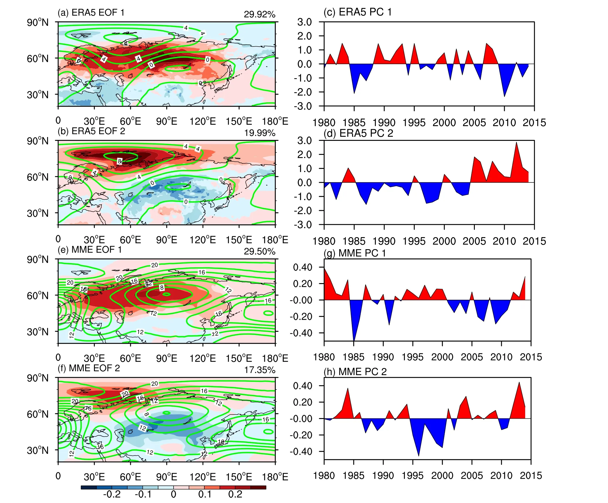
Fig.3.(Left) First and second patterns (EOF1 and EOF2) and (right) their principal components (PC1 and PC2) of the winter SAT in Eurasia (20°–90°N, 0°–180°E) during the time period 1980–2014 in (a–d) the ERA5 dataset and(e–h) the MME.The solid green contours represent the winter Z500 difference between 2005–14 and 1980–2004.

Our analysis shows that there are differences in the ability of each model to simulate the WACE pattern, but understanding the reasons for the differences requires analysis.We therefore searched for the reasons using group comparisons.First,we used the definition of Taylor to calculate the S value of the climatology or the standard deviation of the winter SAT in Eurasia simulated by the 39 CMIP6 models (Table S1 in the ESM).We then divided the 39 models into two groups based on their ability to simulate the climatology: high-S value models (Cli_HS) and low-S value models (Cli_LS).We also divided the two models into two groups according to their ability to simulate the standard deviation: Std_HS and Std_LS models.We then combined these groups into four groups: Cli_HS/Std_HS, Cli_HS/Std_LS, Cli_LS/Std_HS, and Cli_LS/Std_LS (Table 2).The top ten models according to the ranking of their ability to simulate the WACE pattern were defined as WACE_HS; the bottom ten models were WACE_LS and the rest were defined as WACE_MC (Table S1).

Figure 7 compares the percentages of WACE_HS,WACE_MC, and WACE_LS in the four groups of models(Cli_HS/Std_HS, Cli_HS/Std_LS, Cli_LS/Std_HS, and Cli_LS/Std_LS).The four columns on the left show that WACE_HS accounts for the highest percentage (50.0%) in the Cli_HS/Std_HS group, whereas it only accounted for 11.1% in the Cli_LS/Std_LS group.This shows that when the climatology and standard deviation are simulated well,the WACE pattern can also be simulated well.By contrast,if the simulation results of the climatology and standard deviation are not good, then the results for the WACE pattern are also poor.

To investigate these results further, we denoted the Cli_HS/Std_HS and Cli_LS/Std_LS groups of models as HS and LS, respectively (Table 2).We made a comparison of SAT climatology and variability between HS and LS models (Fig.8).The HS models obviously show a climatology and variability much closer to observation.Figure 9 shows the MME of the EOF2 of the two groups (HS/LS).We compared their simulation capabilities for EOF2–that is, we compared Fig.9 (HS/LS), Fig.3f (MME), and Fig.3b (ERA5).Both HS and LS simulated the spatial distribution of the WACE pattern, but the EOF2 (WACE pattern) simulated by HS was more consistent with the ERA5 dataset (Fig.9a).However, the range of the warming center simulated by LS was smaller than when using the ERA5 dataset, and the location was further to the west (Fig.9b).In addition, by calculating the SCC of the three groups and the ERA5 dataset, we found that R(HS) = 0.90, R(LS) = 0.56, and R(MME) = 0.89,showing that the simulation effect of HS on the WACE pattern was much better than that of LS.

Fig.4.Variance explained by (a) EOF1 and (b) EOF2 of the interannual variation in the winter SAT over (20°–70°N, 0°–180°E) in the observations and the CMIP6 Historical simulations during the time period 1979–2014.

Fig.5.Regression coefficients of winter SAT against the normalized PC2 time series during 1979–2014 for the (a) ERA5,(b) MME, and (c) difference between MME and ERA5.The dotted shading indicates the 99% confidence level.

Fig.6.Same as Fig.2, but for regressed winter SAT on normalized PC2 time series during 1979–2014.

Table 2.Grouping results of the 39 models based on their ability to simulate the climatology well (Cli_HS) and poorly (Cli_LS) and to simulate the standard deviation well (Std_HS) and poorly(Std_LS) based on the S index.There are 20 (19) models with a climatological S index greater (less) than 0.93.Similarly, there are 20 (19) models with a standard deviation of the S index greater(less) than 0.63.

Fig.7.Performance of different model groups in simulating the WACE pattern: percentage of WACE_HS (good models;red bars), WACE_MC (medium models; green bars), and WACE_LS (bad models; blue bars) models in the six groups of models (Cli_HS/Std_HS, Cli_HS/Std_LS, Cli_LS/Std_HS,Cli_LS/Std_LS, Std_BKS_HS, and Std_BKS_LS).

Although the simulation results of the climatology by CMIP6 are close to the observations, there are large deviations in the simulation results of the standard deviation (reflecting the extremes), both among the models and between the models and the observations.The proportion of WACE_HS in the group with well-simulated extremes (Cli_HS/Std_HS and Cli_LS/Std_HS) was greater than that in the group with a well-simulated climatology (Cli_HS/Std_HS and Cli_HS/Std_LS).This suggests that, for the simulation of the WACE pattern, simulation of the extremes of the SAT is more important than the simulation of the climatology.

Fig.8.Same as Figs.1b, c, e, and f, but for HS and LS models.

Fig.9.MME of EOF2 of the winter SAT in Eurasia during the time period 1980–2014 based on the (a) HS and (b)LS models in CMIP6.

In addition, the CMIP6 models have some limitations in improving the global and regional SAT and extreme events; even extreme cold events at high latitudes have a stronger cold deviation (Kim and Son, 2020).Of note is that the warm Arctic does not necessarily correspond to cold Eurasia (Luo et al., 2022), and the WACE pattern can be reflected well by the generation of cold extreme events over Eurasia related to UB.Therefore, simulating the BKS warming and the strength and movement of UB is very important for the ability of CMIP6 models in simulating the WACE pattern.

Based on their ability to simulate extremes in the BKS region (70°–90°N, 10°–90°E), we used the S index to divide the 39 modes into two groups (Std_BKS_HS and Std_BKS_LS) and compared the proportions of WACE_HS,WACE_MC, and WACE_LS in the two groups.The results in the two right-hand columns of Fig.7 show that WACE_HS accounted for 40.0% in the Std_BKS_HS models, much higher than the 10.5% in the Std_BKS_LS models.The ability of the CMIP6 models to simulate SAT anomalies in the BKS area therefore affects their ability to simulate the WACE pattern.

We also analyzed the possible reasons for the difference in simulating the SAT anomaly in the BKS region and the associated atmospheric circulation.Figure 10 shows the detrended Z500 (shading) obtained by regression on the WACE time series during the time period 1980–2014.There were three positive anomaly centers in the observational results (the Ural Mountains, the North Pacific, and the North Atlantic), corresponding to areas with frequent blocking.The midlatitudes of Eurasia exhibited a significant negative anomaly (Fig.10a).The distribution of the height anomaly field can therefore be roughly simulated by the MME.

However, there is a gap between the MME and the observations in the simulation of UB, which is mainly manifested in a more westward position and weak intensity (Fig.10b).HS (Fig.10c) can simulate the distribution of the anomaly consistent with the observations; the intensity and location of UB are both closer to the observations than for the MME.In addition, LS (Fig.10d) shows a distribution of positive west and negative east anomalies in the Ural Mountains and Siberia, which is inconsistent with the observations.Combining Figs.9 and 10, the UB in HS can be related to the warming center in the BKS region, whereas the blocking in LS can be related to the warming center in Europe.

Fig.10.Regression coefficients (color) of detrended winter Z500 against the WACE time series during 1980–2014 in the (a) ERA5, (b) MME, (c) HS, and (d) LS and (e) the difference fields between HS and LS.Dots indicate the 90%confidence level.The contours denote the deviation of the composite SAT of (b) MME, (c) HS, and (d) LS from the ERA5 dataset.

In addition, by comparing the difference between the MME, HS, LS, and the observations (Figs.10a–d, respectively), we found that the deviations were largest in the Arctic.Among them, the deviation of LS was greater than that of MME, with the smallest for HS.Previous studies have shown that the stability of UB is conducive to the warming of the Arctic, and the connection between Arctic warming and extreme cold events in the midlatitudes of Eurasia is also related to UB (Luo et al., 2016a; Li and Ren, 2019).It can be inferred from this that the ability of the CMIP6 models to simulate the location and intensity of UB is related to their ability to simulate the WACE pattern.

In observation, the persistence and movement of UB are more important for the WACE pattern than intensity(Yao et al., 2017).Therefore, we further used the daily data of 10 CMIP6 models and NCEP/NCAR to test whether the CMIP6 models of the HS group can simulate duration and movement of UB well.We first calculated the winter blocking frequency (Fig.S2 in the ESM).The result shows that the Ural region is a higher-frequency zone of blocking.Compared with the observation data, the MME of 10 CMIP6 models can simulate the zonal distribution of blocking frequency in the Northern Hemisphere.However, the single CMIP6 models and MME significantly overestimated the frequency of UB, which is consistent with Chen et al.(2021).Compared with Table 2, 6 out of 10 models belong to the HS group,and we synthesized the models in HS.The results show that the HS model group is closer to the observation than the MME.Therefore, we can conclude that UB plays an important role in the WACE pattern.

The ability to simulate UB is further analyzed by time–longitude evolution (Fig.S3 in the ESM).Figure S3a shows that the frequency of blockings in the Ural Mountains is higher than that in other areas of the same latitude.UB frequently appears in late winter (i.e., late January to February).Late January and late February are two periods of high UB frequency.In late winter, the duration of the blockage is about 5–10 days, and UB gradually moves east to near 70°E after it occurs.The MME can simulate the time–longitude characteristics of blocking (Fig.S3b).In the simulation results of the MME and HS models, in general, the UB frequency simulated by the MME is higher, and the position is more eastward.In contrast, the simulation of the blocking frequency in the models of the HS group is improved (Fig.S3c).

Importantly, the ability to simulate persistence of UB is further analyzed by analyzing the relationship between daily UB intensity and temperature anomalies between the BKS and Siberia regions (Fig.11).It can been seen that HS models show more persistent UB and a warmer BKS region and colder Siberia, i.e., the more obvious WACE pattern.

6.Summary and discussion

We evaluated the simulations of CMIP6 models on the climatology, standard deviation, and main mode of the winter SAT in Eurasia over (20°–90°N, 0°–180°E) from 1980 to 2014 and analyzed the reasons for the difference in the ability of the CMIP6 models to simulate the WACE pattern.The CMIP6 models can roughly simulate the spatial distribution of the climatology and standard deviation, but there are large inter-model spreads in the SCC and the normalized standard deviation among the 39 models.The simulation of the climatology is better than that of the standard deviation.The results of the MME are better than the results of most models.For the simulation of climatology, the CMIP6 models generally underestimated the actual SAT, and the deviation reached the maximum of 8°C in the BKS region.The deviation in the simulation of the standard deviation was also largest in the BKS region, reaching 1°C.

Fig.11.Time series of composite daily (a) Z500 anomaly(gpm) averaged over (60°–70°N, 30°–60°E), SAT anomaly (°C) averaged over the BKS region (70°–80°N, 20°–90°E), and SAT anomaly (°C) averaged over the Siberia region (40°–60°N, 60°–110°E) during the UB life cycle for the HS models and the other models.

Through the analysis of the main modes, we found that the MME can simulate the spatial distribution of the main modes consistently with the observations–that is, the MME EOF1 shows uniform warming, and the EOF2 is the WACE pattern.There was also a large gap among the models in simulating the EOF2.We found that this difference was related to the ability of the models to simulate the climatology and standard deviation of the winter SAT over Eurasia during the time period 1980–2014.The simulation of the WACE pattern by the Cli_HS/Std_HS models (with good performance in the climatology and standard deviation) (WACE_HS number accounts for 50%) was significantly better than the simulation by the Cli_LS/Std_LS models (WACE_HS number accounts for only 11.1%).This suggests that the ability of the CMIP6 models to simulate the WACE pattern is related to their ability to simulate the climatology (average value)and extremes (variability).In general, the ability of the CMIP6 models to simulate the climatology was much better than their ability to simulate extremes (variability).We further found that the key atmospheric circulation affecting the simulation performance of the SAT extremes in the BKS region was located in the Ural Mountains.The simulation of the CMIP6 models of the intensity and location of UB affects their ability to simulate the WACE pattern.The warm and wet advection behind UB is transported to the Arctic, forming a warm anomaly in the BKS region.Cold advection in front of UB can cause cold anomalies in central and eastern Asia (e.g., Luo et al., 2016a; Dong et al., 2020),which is conducive to the appearance of the WACE pattern.The difference sequence of Z500 between the Ural Mountains(50°–75°N, 50°–110°E) and Europe (50°–75°N, 0°–50°E)(the blue curve in Fig.12) is significantly correlated with the observed temperature PC2 (the red curve in Fig.12) (r =0.37, P < 0.05).This result proves that winters dominated by Ural (European) blocking do easily (not easily) show the WACE pattern.We synthesized the SAT anomalies in the winters dominated by UB blockings (the positive center of Z500 located within 50°–75°N and 50°–110°E) and winters dominated by European blockings (the positive center of Z500 located within 50°–75°N, 0°–50°E) based on the ERA5 dataset and the CMIP6 HS (Cli_HS/Std_HS) and LS(Cli_LS/Std_LS) models, respectively (Fig.13).In the ERA5 dataset, when UB was dominant, warm air was located in the BKS region, and cold air was present in Eastern Siberia and East Asia (Fig.13a).By contrast, when European blocking dominated, warm air was more to the west and accumulated in Scandinavia.At this time, the BKS region was occupied by strong cold air, which is not conducive to the emergence of the WACE pattern (Fig.13b).In the CMIP6 models, the HS group can simulate the results better than the LS group (Figs.13c–f).This shows that accurately simulating the location and strength of UB is very important in simulating the WACE pattern.It determines the location of cold and warm air and, in turn, the formation of the WACE pattern.That is to say, if the models can simulate the warm anomaly in the BKS area and the height field in the Urals,then they can usually also simulate the WACE pattern well.Therefore, by improving the ability of the CMIP6 models to simulate UB, we can also improve the simulation of the extreme winter SATs in Eurasia and the BKS region and, in turn, the ability of the CMIP6 models to simulate the WACE pattern.

This conclusion is different from that drawn from the CMIP5 models (Wang et al., 2020).The reason why the CMIP5 models are not good at simulating the WACE pattern is often considered to be due to their poor simulation of the loss of SIC, especially the magnitude of the loss (e.g., Wang et al., 2020), although some CMIP5 models can exhibit a non-linear response of circulation to SIC decrease (Yang and Christinsen, 2012).Through the evaluation of CMIP6 in this study, we found that the simulation performance of UB can directly affect the simulation effect of the SAT anomaly in the BKS region and midlatitude and high-latitude Asia, which, in turn, affects the simulation of the WACE pattern.The performance depends more on the simulation of the variability than the simulation of the average.

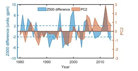
Fig.12.Difference sequence (blue) of detrended winter Z500 (units: gpm) between the Ural Mountains (50°–75°N, 50°–110°E) and Europe (50°–75°N, 0°–50°E) and the second principal component sequence (PC2; red) of the winter SAT (based on the ERA5 dataset).The gray dashed lines mark 0.5/–0.5 times the standard deviation of the Z500 difference sequence, regarded as the winters dominated by the UB/the European blocking.

Fig.13.Composite SAT anomalies (units: °C) in winters dominated by (left) UB and (right) European blocking.(a and b) Based on the ERA5 dataset.(c and d) Based on the CMIP6 HS models.(e and f) Based on the CMIP6 LS models.Green dots indicate the 90% confidence level.

On the other hand, the BKS sea ice may be considered as an independent forcing of atmospheric circulation.Some studies suggest that SIC reduction, through a changed atmospheric circulation, largely and independently contributed to cold winters in Central Eurasia (Petoukhov and Semenov,2010; Mori et al., 2014; Semenov and Latif, 2015).The reason for this is likely to be that the sea ice and temperature in the BKS region in winter are usually controlled by the oceanic heat inflow (e.g., Schlichtholz, 2011, 2013).So, we examined a dependence of the WACE pattern in CMIP6 models on BKS sea ice.We compared the performances of simulating the relationship between the WACE pattern and SIC for the two new groups of HS and LS models, which have different abilities to simulate SIC climatology and variability (Fig.S4 in the ESM).It shows that the new HS models of SIC have better performance in simulating the relationship between the WACE pattern and SIC than the LS models of SIC.The results suggest that the sea ice likely also has an impact on simulation of the WACE pattern.However, in order to further investigate the role of SIC simulation on the WACE pattern,we plotted regression coefficients of SAT against the WACE pattern time series in the different groups and the difference fields using the new HS and LS groups chosen according to SIC simulation ability (Fig.S5).It shows that the HS models simulating sea ice well do not reproduce a better WACE pattern than LS models.

Although our study reveals that the simulation of the WACE pattern usually depends on the ability to simulate UB events and SIC, sea surface temperature in the North Atlantic and Pacific may also modulate the WACE pattern via the Atlantic Multidecadal Oscillation (AMO) and Pacific Decadal Oscillation (PDO) (Jin et al., 2020; Luo et al., 2022).However, the ability of CMIP6 models to simulate the relationship between the AMO, PDO, and WACE pattern is unclear and needs further investigation.

Acknowledgements.We acknowledge the World Climate Research Program’s Working Group on Coupled Modeling and thank the climate modeling groups for producing and making available their model output.This research is supported by the National Natural Science Foundation of China (Grant Nos.41790471,42075040, and U1902209), the Strategic Priority Research Program of the Chinese Academy of Sciences (XDA20100304), and the National Key Research and Development Program of China(2018YFA0606203, 2019YFC1510400).

Data availability.All the data used in this study is available at https://cds.climate.copernicus.eu/ and https://esgf-node.llnl.gov/projects/cmip6/.

Electronic supplementary material:Supplementary material is available in the online version of this article at https://doi.org/10.1007/s00376-022-2201-4.