Yang Shi| Qiaowen Shi | Xinwei Cao | Bin Li | Xiaobing Sun |Dimitrios K.Gerontitis

1School of Information Engineering, Yangzhou University,Yangzhou, China

2Jiangsu Province Engineering Research Center of Knowledge Management and Intelligent Service,Yangzhou University, Yangzhou, China

3School of Business,Jiangnan University,Wuxi,China

4Department of Information and Electronic Engineering,International Hellenic University,Thessaloniki, Greece

Abstract Time-varying matrix inversion is an important field of matrix research, and lots of research achievements have been obtained.In the process of solving time-varying matrix inversion,disturbances inevitably exist,thus,a model that can suppress disturbance while solving the problem is required.In this paper, an advanced continuous-time recurrent neural network (RNN) model based on a double integral RNN design formula is proposed for solving continuous time-varying matrix inversion, which has incomparable disturbance-suppression property.For digital hardware applications, the corresponding advanced discrete-time RNN model is proposed based on the discretisation formulas.As a result of theoretical analysis,it is demonstrated that the advanced continuous-time RNN model and the corresponding advanced discrete-time RNN model have global and exponential convergence performance, and they are excellent for suppressing different disturbances.Finally, inspiring experiments, including two numerical experiments and a practical experiment,are presented to demonstrate the effectiveness and superiority of the advanced discrete-time RNN model for solving discrete time-varying matrix inversion with disturbance-suppression.

K E Y W O R D S neural control, neural network, real-time systems

1 | INTRODUCTION

Matrix is one of the main contents of linear algebra in mathematics.It is simple and effective to solve many practical problems using matrix ideas.Matrix inversion is an important field of matrix theory, and it is used as a basic mathematical tool in scientific and engineering researches, such as robot manipulator control[1],radar[2],and mathematical models[3].In view of this, people are devoted to finding efficient matrix inversion methods.

Generally,appropriate processing methods are selected according to the solution scale and problem characteristic.Usually,there are two categories of methods for matrix inversion:direct methods and iterative methods.Among them, Gaussian elimination, lower-upper decomposition, and singular value decomposition are typical direct methods, which compute the exact solution without residual errors through row-column transformation and other operations in the matrix.Alternatively,an iterative approach is to consider the matrix inversion from the view of equation,starting from a given initial value and recursively computing the next value,which is more suitable for large-scale matrices.For example,for the solution of non-linear equations with many variables, which also contain matrix inversion, the cost of taking direct methods is too high, and iterative methods are usually used.Note that, although the majority of existing algorithms deal with static problems, in reality [4–6], time-varying systems and problems frequently develop,making conventional algorithms inapplicable.

Neural networks have achieved widespread success in artificial intelligence, automated control, signal processing,and many other research areas [7–9].It acts like a brain,describing behaviour through rigorous mathematical derivation and flexible use of knowledge.Note that, in recent years,the recurrent neural network (RNN) plays a key role and becomes the research focus of researchers [10–23].Zeroing neural network (ZNN) is a special RNN model created by Zhang et al.[13–15], which is designed for handling timevarying problem by using the derivative information of time-varying parameter.In the above study, researchers have proposed and studied lots of models for solving time-varying matrix inversion.For example, in Ref.[22], an improved varying-parameter ZNN model including time-varying design parameter was proposed, which can calculate the matrix inversion in real-time, and the robustness of the model was enhanced by rapidly increasing the value of the parameters in the model.In Ref.[23], a unified gradient neural network model with a simple structure was proposed to deal with static matrix inversion and time-varying matrix inversion, and it converged in finite time.

However, disturbances inevitably exist in practice, and there have been a lot of studies on how to suppress disturbance in the process of solving the problem.Many methods have been proposed that do not require additional disturbancesuppression modules.For example, a new RNN design formula for solving time-varying matrix inversion was constructed, and the disturbances in different cases can be suppressed simultaneously in Ref.[24].Similarly,in Ref.[25],a prescribed-time convergent and noise-tolerant Z-type neural dynamics model that uses the novel design formula and function was proposed, and the theoretical analyses showed that the model had convergence and better anti-noise ability.Besides, a kind of ZNN that can suppress complex-valued disturbances was proposed to solve the problem of complexvalued time-varying matrix inversion with various noise conditions in Ref.[26], which made use of integral control techniques from the proportional-integral-derivative(PID)control system [27–31].Generally speaking, the models studied in the above references are effective to overcome the disturbance problem.

In addition, for the purpose of digital hardware implementation, such as digital circuit, digital computer, and numerical algorithm, researchers began to focus on the development of corresponding discrete-time models for solving time-varying problems [32–39].For example,in Refs.[35, 36],Euler forward differences were used to construct discretisation continuous-time RNN models; in Ref.[38], a new numerical difference rule of first derivative approximation based on Taylor series expansion was established, and two new discrete-time RNN (DT-RNN) models were proposed based on this rule;in Ref.[39], in order to replace the traditional static solver and for the time-varying matrix inversion, two discrete-time models that can suppress constant disturbance, random disturbance, and discrete time-varying linear disturbance were constructed.

Although there have been some achievements in combining DT-RNN models for solving time-varying matrix inversion,the research on combining discretisation methods to solve the problem is far from complete.Typical research results are presented in Table 1.Specifically, first of all, as shown in Table 1, the traditional continuous-time RNN (T-CT-RNN)model was presented for solving time-varying matrix inversion in Ref.[40], but such a model cannot suppress disturbance in real-time; secondly, the integration-enhanced continuous-time RNN (IE-CT-RNN) model was presented in Ref.[24] for solving time-varying matrix inversion with various disturbances, but it hardly suppresses time-varying quadratic disturbance during the inverse matrix solution.Note that, in the above references, the T-CT-RNN model and the IE-CTRNN model do not consider discretisation.In addition, in the research of discrete-time model, a DT-RNN model was presented in Ref.[41] for solving time-varying matrix inversion, but the suppression of the disturbance was also not considered.Evidently, the mentioned inadequacies of these studies highlight the importance of this paper.

The following sections of this paper are divided into five sections.In Section 2, the problem formulation and the advanced continuous-time RNN(A-CT-RNN)model are presented, and related two traditional models (i.e., IE-CT-RNNand T-CT-RNN model)are also presented for comparison.In Section 3, the theoretical analyses are presented, which show that the state solution of the proposed A-CT-RNN model converges globally and exponentially to the theoretical solution of time-varying matrix inversion and that it remains convergent in the presence of different kinds of disturbances.In a series of theoretical analyses, Section 4 presents the advanced DT-RNN (A-DT-RNN) model and shows that the state solution of the proposed A-DT-RNN model converges globally and exponentially to the theoretical solution of discrete time-varying matrix inversion with excellent capacity for suppressing disturbance.In Section 5, the comparative numerical experimental results of the A-DT-RNN model, the traditional DT-RNN (T-DT-RNN) model and the integration-enhanced DT-RNN (IE-DT-RNN) model are presented, and this section also presents a kinematic control application of a manipulator to further validate the proposed A-DT-RNN model.The conclusions of this paper are found in Section 6.As a result of this paper, the following contributions are presented.

T A B L E 1 Comparison of related methods.

• In this study,a novel RNN design formula is proposed and studied, which is an improvement on the traditional design formula [24] proposed by Jin et al.

• Based on the novel RNN design formula,we propose an ACT-RNN model and an A-DT-RNN model for solving time-varying matrix inversion.In order to verify the ability of models to suppress disturbance,the problem is solved in the presence of different disturbances.It is noteworthy that this is the first time a neural network model that can suppress continuous time-varying quadratic disturbance for solving continuous time-varying matrix inversion has been proposed.

• Furthermore,we present theoretical analyses and results that ensure the global and exponential convergence of the ADT-RNN model for solving discrete time-varying matrix inversion and further demonstrate that the A-DT-RNN model has the ability to suppress disturbance.

• Under different disturbances, especially discrete timevarying quadratic disturbance, numerical experiments demonstrate the effectiveness and superiority of the A-DTRNN model for solving discrete time-varying matrix inversion with disturbance-suppression.

The following list summarises the mathematical symbols used in this study.

Mathematical symbols

(Continued)

2 | PROBLEM FORMULATION AND A‐CT‐RNN MODEL

Note that, for the discrete time-varying matrix inversion, we first consider the continuous-form of the problem as shown in this section and then we define the continuous time-varying error function and use the novel RNN design formula to establish the A-CT-RNN model.

2.1 | Problem formulation

The problem formulation of the continuous time-varying matrix inversion is defined as

whereX(t)∈Rn×nis an unknown matrix to be solved,I∈Rn×nis an identity matrix, andA(t)∈Rn×nis a nonsingular smooth time-varying matrix.The purpose of this equation is to efficiently obtain the inverse ofA(t),which isX(t),in real-time from the given values ofA(t) andI.Furthermore,the problem formulation of the discrete time-varying matrix inversion is defined as

In this study, we start with a continuous time-varying matrix inversion, and in the subsequent discrete time-varying matrix inversion, we havetk+1fort((k+1)g),wheregrepresents the step size.

2.2 | A‐CT‐RNN model

Next, continuous time-varying matrix inversion can be monitored using the following error function:

Then, the time derivative can be described as follows:

whereλ> 0,μ> 0 andν> 0 are three designed parameters that can affect the convergence speed of the A-CT-RNN model.According to the error function and the novel RNN design Formula(3), the implicit neural network model, that is,the A-CT-RNN model, can be obtained as follows:

To evaluate the performance of(4)with different disturbances,the proposed A-CT-RNN model (4) is affected by unknown disturbance, and the equation becomes

whereW(t)∈Rn×ndenotes time-varying matrix-form disturbance.

2.3 | Other models

For comparison purposes, the following description equation for the implicit dynamics of the T-CT-RNN model [40] to solve continuous time-varying matrix inversion is directly given as

Besides, the following description equation for the implicit dynamics of the IE-CT-RNN model [24] to solve continuous time-varying matrix inversion is directly given as

When the T-CT-RNN model (6) is affected by unknown disturbances, the equation becomes

and similarly when the IE-CT-RNN model (7) is affected by unknown disturbances, the equation becomes

and as shown in the above equation,W(t)∈Rn×ndenotes time-varying matrix-form disturbance.

3 | THEORETICAL ANALYSES OF A‐CT‐RNN MODEL

In this section, for solving continuous time-varying matrix inversion,first of all,two theorems are given to presentthe global and exponential convergence properties of the A-CT-RNN model (4).Secondly, three theorems are given to present the convergence of the state solution of the A-CT-RNN model(4)to the theoretical solution of continuous time-varying matrix inversion(1)with different disturbances.

Theorem 1.The state solution of the A-CT-RNN model(4)globally converges to the theoretical solution of continuous time-varying matrix inversion(1)with appropriate parameters.

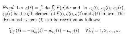
Proof.In the case ofE(t),leteij(t)be theijth element,where ∀i,j= 1, 2, …,n.The dynamical system (3) can be rewritten as follows:

Thereinto,λ,μandνin (3) correspond to the coefficients of the various items in (10), that is,λ=k1+k3,μ=k2+k1k3andν=k2k3,and we setk1>0,k2>0 andk3>0.Note that the appropriate parameters should be selected, which can be seen as a future research direction.

First of all,an error function is defined to demonstrate the theorem as

According to the classical ZNN design formulation, the following equation can be further defined as

Obviously,zij(0) =eij(0) and ˙zij(0)=-k3eij(0), and the Lyapunov function candidate function of theijth subsystem(12)is defined as

In addition, the time derivative of the above equation is expressed as follows:

Clearly,vij(t) > 0 whenzij(t) ≠0, andvij(t) = 0 only whenzij(t) = 0.As a result, the positive definiteness ofvij(t) is guaranteed by this.Combined with ˙vij(t)≤0, according to Lyapunov theory,it follows thatzij(t)of theijth subsystem(12)converges to zero globally.

Substituting the Equation (11) into the Equation (12), the following formula can be obtained,namely,the Equation(10):

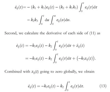
Through the above deduction, we transform Equation (10)with double integral into Equation (13) with single integral.Therefore,we only need to prove thateij(t)globally converges to zero, and then this theorem can be proved.

Next,the Lyapunov function candidate function of theijth subsystem (13) is defined as

In addition, the time derivative of the above equation is expressed as follows:Clearly,vij(t) > 0 wheneij(t) ≠0, andvij(t) = 0 only wheneij(t) = 0.As a result, the positive definiteness ofvij(t) is guaranteed by this.Based on Lyapunov theory and combined with ˙vij(t)≤0, it follows thateij(t) of theijth subsystem (13)converges to zero globally, and this implies thatE(t) globally converges to zero.

In conclusion, the state solution of the A-CT-RNN model(4) globally converges to the theoretical solution of (1).The proof is thus completed.□

In addition, considering the use of integrals in Theorem 1,the description ofeij(t) needs to be presented, and to further study the convergence ofE(t), the following theorems are proposed.

Theorem 2.The state solution of the A-CT-RNN model(4)exponentially converges to the theoretical solution of continuous time-varying matrix inversion(1).

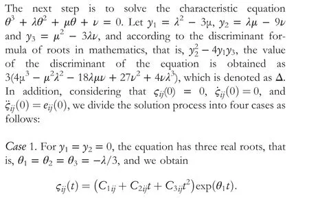
Note that the values ofC1ij,C2ijandC3ijin the above equation are obtained according to the initial trial conditions.Then, we further obtainA

s a result of taking two derivatives,it is possible to generalise the error description formula as follows:

Case2.ForΔ> 0, there are one real root and two complex conjugate roots inθ1,θ2andθ3.Supposeθ1is a real root,and

As a result of taking two derivatives,it is possible to generalise the error description formula as follows:

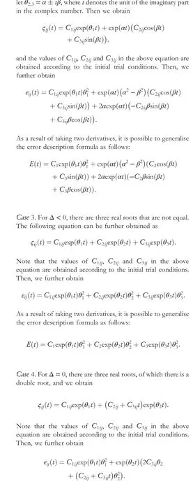
Summarising the above four cases and based on Theorem 1,it appears that the state solution of the A-CT-RNN model (4)converges exponentially to the theoretical solution of (1),whatever the initial conditions are.The proof is thus completed.□Next, three theorems are used to investigate the A-CTRNN model (4) with constant disturbance, continuous timevarying linear disturbance, and continuous time-varying quadratic disturbance.

Theorem 3.The state solution of the A-CT-RNN model(4)affected by the constant disturbance W(t)=W∈Rn×n gradually converges towards the theoretical solution of(1).

Proof.According to the Laplace transformation, (5) can be transformed as follows:

Evidently, given thatλ> 0,μ> 0 andν> 0, in order for the denominator not to be zero,that is,s3+λs2+μs+ν≠0,the solution iss1<0,s2<0 ands3<0.Due to the location of the three poles in the left half plane, the system is stable.The following result can be derived from the final value theorem[42]:

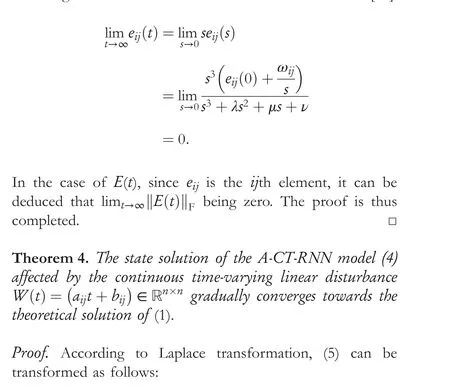
The stability of this system can be proved in a similar way as shown in the above-mentioned theorem.Based on the final value theorem [42], we further obtain the following equation:

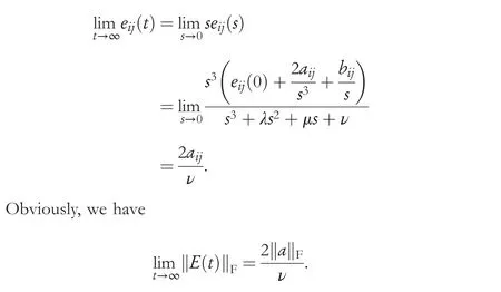
The proof is thus completed.□

4 | A‐DT‐RNN MODEL AND THEORETICAL ANALYSES

The A-DT-RNN model is investigated and developed in this section, and through the corresponding theoretical analyses, it is concluded that the proposed A-DT-RNN model is 0-stable,consistent and convergent.

4.1 | Correlation formula

In order to provide two formulas that can be used with the discretisation model, a lemma and a theorem are presented in this subsection.

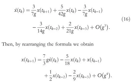
Lemma 1.According to Ref.[43],the 5-instant discretisation formula is formulated as follows:The function of this formula is to discretise the proposed ACT-RNN model (4).

Next, considering the double integral term for the A-CTRNN model (4), we propose the following theorem to obtain its approximation.

Theorem 6.Based on Taylor expansion,a novel one-step forward difference formula for double integral approximation is defined:

where ¨f(tk) represents the second derivative off(tk).The proposed new difference formula can achieve better computational performance in RNN discretisation, which is specifically shown in Subsection 4.2.

Proof.Note thatk+istands for(k+i)g,wheregstands for the step size.By Taylor expansion,the following formulas can be obtained:wherec1,c2,c3andc4are real numbers betweenkandk+ 1.The following formulas can be obtained by rearranging the above formulas as

Then, through the algebraic operation “11 × (18) + 6 ×(19)+16×(20)-9×(21)”.The proof is thus completed.□

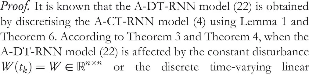
4.2 | A‐DT‐RNN model and other models

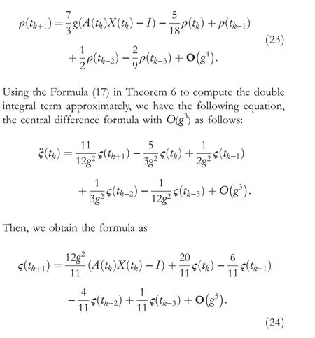
Using the discretisation Formula(16)as a basis for discretising the A-CT-RNN model (4), the A-DT-RNN model is generated as follows:

As in the previous equation,termsρ(tk)andζ(tk)represent the single integral term and double integral term, respectively.Their numerical approximation formulas are described below.

Calculating the single integral term approximately using the discretisation Formula(16),the equation can be summarised as follows:

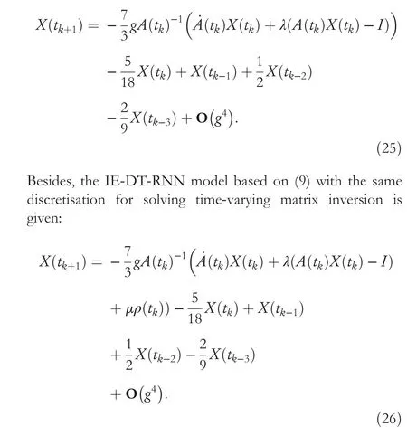
In addition, for comparison purposes, the T-DT-RNN model based on (8) with the same discretisation for solving timevarying matrix inversion is given:

4.3 | Theoretical analyses of A‐DT‐RNN model

The convergence performance of the proposed A-DT-RNN model (22) with constant disturbance, discrete time-varying linear disturbance, and discrete time-varying quadratic disturbance are analysed theoretically as follows.

Theorem 7.The proposed A-DT-RNN model(22) is 0-stable.Proof.By transposing terms,the Formula(22)can be rewritten as

The root of above equation can be obtained, that is,θ1= 1,θ2=0.2976,θ3=-0.7877-0.3552i,θ4=-0.7877+0.3552i.

There are roots on or within the unit circle, which indicates that the proposed A-DT-RNN model (22) is 0-stable.The proof is thus completed.□

Theorem 8.The proposed A-DT-RNN model(22)is consistent and convergent,and its truncation error converges with orderO(g4).

Proof.It can be observed that the truncation error in the expression of the A-DT-RNN model (22) isO(g4), where the truncation error of the single integral approximation (23) as shown below isO(g4):

5 | NUMERICAL EXPERIMENTS AND VERIFICATIONS

In this section, three examples are presented to verify the efficiency of the proposed A-DT-RNN model (22) in the presence of different disturbances.

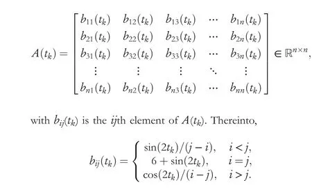
To begin,let us definek+ias(k+i)g,wheregrepresents the step size, and the discrete time-varying Toeplitz matrixA(tk) is considered as follows:

Three models are presented for solving the matrix inversion for comparison after setting the values ofnto two and four,respectively.

5.1 | Example 1

As an example to demonstrate the effectiveness and superiority of the A-DT-RNN model (22), the following discrete timevarying matrix is presented:

Result 1.(Convergence)Figure1illustrates the experimental results of the proposed A-DT-RNN model(22).In detail,using four randomly generated initial states as a starting point and using λ=10,μ=40,ν=50and g=0.01,the state solution of the A-DT-RNN model(22)(as shown in the figure by the blue dashed line)gradually approaches the theoretical solution of(1),as shown in Figure1a.Besides,Figure1bshows that the residual errors of the A-DT-RNN model(22)converge and approach zero in the way of O(g4),and two sets of values are used,λ= 10,μ= 10,ν= 10,g= 0.01;λ= 100,μ= 100,ν= 100,g=0.001.It is observed that the residual errors are found to show different trends for different values of g.Specifically,when g is decreased by a factor of 10,the residual errors decreases by a factor of ten thousand.As aresult of these results,the A-DT-RNN model(22)has proven to be both effective and superior for solving discrete time-varying matrix inversion.

F I G U R E 1 Experimental results of the proposed A-DT-RNN model (22)to solve discrete time-varying matrix inversion.(a)Trajectory solved by the ADT-RNN model (22) with λ = 10, μ = 40, ν = 50 and g = 0.01 in Example 1.(b) Residual errors E(tk+1)‖ ‖F of the A-DT-RNN model (22) with different parameter values,that is,λ=10,μ=10,ν=10,g=0.01 and λ=100,μ=100,ν=100,g=0.001,respectively in Example 1.(c)Residual errors ‖E(tk+1)‖F of the A-DT-RNN model (22) with different parameter values, that is, λ = 10, μ = 10, ν = 10, g = 0.01 and λ = 100, μ = 100, ν = 100, g = 0.001, respectively in Example 2.

F I G U R E 2 Residual errors of T-DT-RNN model(25),IE-DT-RNN model(26),and A-DT-RNN model(22)with constant disturbance W(tk)and different parameter values.(a)With λ=10,μ=80,ν=80,g=0.01 and W(tk)=[20,20]2×2.(b)With λ=100,μ=800,ν=800,g=0.001 and W(tk)=[20,20]2×2.(c) With λ = 100, μ = 800, ν = 800, g = 0.001 and W(tk) = [100, 100]2×2.

F I G U R E 3 Residual errors of T-DT-RNN model(25),IE-DT-RNN model(26),and A-DT-RNN model(22)with discrete time-varying linear disturbance W (t k)= atk+b,atk+b]2×2 to solve discrete time-varying matrix inversion in Example 1,where disturbance parameter values a=2 and b=5.(a)With λ=10,μ=80,ν=80,g=0.01,a=2 and b=5.(b)With λ=100,μ=800,ν=800,g=0.001,a=2 and b=5.(c)With λ=100,μ=800,ν=800,g=0.001,a=10 and b = 20.

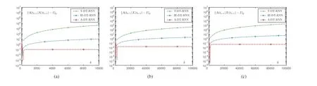
F I G U R E 4 Residual errors of T-DT-RNN model (25), IE-DT-RNN model (26), and A-DT-RNN model (22) with discrete time-varying quadratic disturbance W (t k)= at2k+b,at2k+b to solve discrete time-varying matrix in Example 1.(a) With λ = 10, μ = 80, ν = 80, g = 0.01, a = 2 and b = 20.2×2(b) With λ = 100, μ = 800, ν = 800, g = 0.001, a = 2 and b = 20.(c) With λ = 100, μ = 800, ν = 800, g = 0.001, a = 10 and b = 50.

Result 2.(Constant disturbance)In the actual situation,disturbances inevitably exist,so we add the constant disturbance W(tk)to verify the performance of the A-DT-RNN model(22)in the numerical experiments.To better verify theperformance of the A-DT-RNN model(22),as shown in Figure2,the experimental results are compared among the three models with the same parameter values.In detail,the three sets of parameter values are as follows:λ= 10,μ= 80,ν= 80,g= 0.01and W(tk) = [20, 20]2×2;λ= 100,μ= 800,ν= 800,g= 0.001and W(tk) = [20, 20]2×2;λ= 100,μ= 800,ν= 800,g= 0.001and W(tk) = [100,100]2×2.In addition,the experimental results obtained bytaking the values of the first set of parameters,the second set of parameters.and the third set of parameters are shown in Figure2a–c,respectively.Obviously,it can be observed thatthe residual errors‖E(tk)‖F=‖A(tk)X(tk)-I‖Fof thethree models eventually tend to be stable with the increase of time,which indicates that they all have the ability to suppress constant disturbance,and the suppression effects of the IE-DTRNN model(26)and the A-DT-RNN model(22)are significantly better than those of the T-DT-RNN model(25).

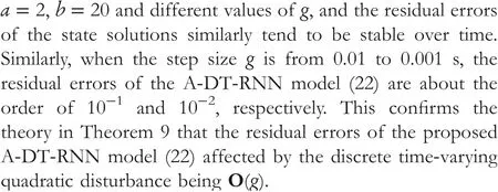
Result 3.(Linear disturbance)Here,we perform numerical experiments by adding the discrete time-varying linear disturbance to verify the performance of the A-DT-RNN model(22).In Figure3,experimental results are shown for the three models.The value of each parameter of the discrete time-varying linear disturbance in matrix form is set to atk+b.Specifically,three sets of parameter values are used:λ= 10,μ= 80,ν= 80,g= 0.01,a= 2and b= 5;λ= 100,μ= 800,ν= 800,g= 0.001,a= 2and b= 5;λ= 100,μ= 800,ν= 800,g= 0.001,a= 10and b= 20,and the experimental results obtained are shown in Figure3a–c,respectively.First,it can be observed that only the residual errors of the IE-DT-RNN model(26)and the ADT-RNN model(22)eventually become stable with the increase of time,which indicates that the T-DT-RNN model(25)cannot suppress discrete time-varying linear disturbance.Then,the final stable residual errors of the IEDT-RNN model(26)are much larger than those of the ADT-RNN model(22),which can confirm that for discrete time-varying linear disturbance,the effect of the A-DT-RNN model(22)on disturbance-suppression is better.

Result 4.(Quadratic disturbance)The experimental results of the A-DT-RNN model(22),the IE-DT-RNN model(26),and the T-DT-RNN model(25)for solving the problem(1)with thediscretetime-varyingquadraticdisturbance Wtk=at2k+b,at2k+b2×2are shown in Figure4.Obviously,only the residual errors of the A-DT-RNN model(22)eventually tend to be stable with the increase of time in the time range shown in the figure,which indicates the ADT-RNN model(22)has an excellent ability to suppress discrete time-varying quadratic disturbance,which is not possessed by the other two models.As illustrated in Figure4a,when g= 0.01,the residual errors of the T-DTRNN model(25)and the IE-DT-RNN model(26)tend to increase with time,while the residual errors of the A-DTRNN model(22)rapidly converge to zero in a short period of time,maintaining the order of 10-1.In addition,in Figure4b,when g= 0.001and the parameter values of the disturbance matrix are set to a= 2and b= 20,the residual errors of the A-DT-RNN model(22)rapidly converge to zero in a short period of time,maintaining the order of 10-2.In Figure4c,when g= 0.001and the parameter values of the disturbance matrix are set to a= 10and b= 50,the residual errors of the A-DT-RNN model(22)also rapidly converge to zero in a short period of time,maintaining the order of 10-2.

These numerical experiments confirm the effectiveness and superiority of the A-DT-RNN model (22) for solving time-varying matrix inversion with disturbance-suppression.

5.2 | Example 2

To further verify the effectiveness of the A-DT-RNN model(22), the following time-varying Toeplitz matrix is considered:

Next, the A-DT-RNN model (22) is used to solve the inverse of the matrixA(tk)in Example 2,and the trajectory of the state solution of the inverse of the matrix in Example 2 solved by the A-DT-RNN model(22)is shown in Figure 1c.Specifically,using four randomly generated initial states as a starting point,Figure 1c shows that the residual errors of the A-DT-RNN model (22) converge and approach zero in the way ofO(g4),and two sets of parameter values are used:λ= 10,μ= 10,ν= 10,g= 0.01;λ= 100,μ= 100,ν= 100,g= 0.001.

5.3 | Example 3

This paper presents a kinematic control application of a manipulator to further validate the proposed A-DT-RNN model (22).By calculating the inverse of the discrete timevarying Jacobian matrix, the proposed A-DT-RNN model(22) is applied to control the motion of the two-link manipulator, and the motion path is plotted.Compared with the desired path,the position errors of the actual trajectory can be used to determine the validity of the proposed A-DT-RNN model (22).

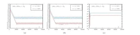
Initially,the robot arm is set to follow an elliptic curve for 30 s with arms that measure 1 m in length and joint angles ofπ/19 andπ/3.The IE-DT-RNN model(26)is initially utilised for comparison,and Figure 6a shows the path of the robot arm tracking ellipse with the blue curve representing the desired path and the red curve representing the actual trajectory.It can be clearly observed that the actual trajectory diverges from the desired path and does not follow it.Figure 6b gives a clearer picture of the actual trajectory and the desired path.Figure 6c shows the position error.It is found that the error increases slowly with time and is not stable.It can be verified that the IE-DT-RNN model(26)does not perform well in suppressing discrete time-varying quadratic disturbance.

Then,the path of the manipulator tracking ellipse is shown in Figure 7a using the proposed A-DT-RNN model (22)affected by discrete time-varying quadratic disturbance with the blue curve representing the desired path and the red curve representing the actual trajectory.It is obvious to observe that the actual trajectory is very close to the desired path.The clearer picture of the actual trajectory and the desired path are shown in further detail in Figure 7b.The position error is depicted in Figure 7c.The maximum error is not more than 10-1, and the error fluctuates steadily with time.The effectiveness and superiority of the A-DT-RNN model (22) are further verified by the numerical experiments of manipulator motion control, which prove that it has the ability to suppress discrete time-varying quadratic disturbance.

F I G U R E 5 Experimental results of the A-DT-RNN model (22) to solve discrete time-varying matrix inversion in Example 2 with different disturbances and different parameter values,that is,λ=10,μ=80,ν=80,g=0.01 and λ=100,μ=800,ν=800,g=0.001,respectively.(a)With constant disturbance W(tk) = [20, 20]2×2.(b) With discrete time-varying linear disturbance W (tk )=tk+b,atk+b]2×2 using a = 2 and b = 5.(c) With discrete time-varying quadratic disturbance W (t k)=using a = 2 and b = 20.

F I G U R E 6 Application of the IE-DT-RNN model (26) to control the two-link manipulator with discrete time-varying quadratic disturbance W (t k)= at++b2×2 using a=0.1,b=0.5,λ=10,μ=40,ν=50 and g=0.01.(a)Kinematic path of the two-link manipulator.(b)Actual trajectory of end effector and desired path of end effector.(c) End effector position error.

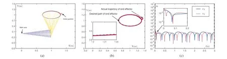
F I G U R E 7 Application of proposed A-DT-RNN model (22) to control the two-link manipulator with discrete time-varying quadratic disturbance W (tk )=at2k+b using a=0.1,b=0.5,λ=10,μ=40,ν=50 and g=0.01.(a)Kinematic path of the two-link manipulator.(b)Actual trajectory of end effector and desired path of end effector.(c) End effector position error.

6 | CONCLUSION

In this study,for solving time-varying matrix inversion,a novel A-DT-RNN model(22)is proposed,analysed and investigated.First of all,we propose a novel RNN design formulation(3)to solve continuous time-varying matrix inversion with different disturbances,and based on the novel design formulation(3),the A-CT-RNN model (4) is proposed and studied.Then, using the discretisation Formula (16) to discretise the A-CT-RNN model (4), the A-DT-RNN model (22) is generated.In addition,according to the theoretical analyses,the A-CT-RNN model(4)and the A-DT-RNN model(22)both exhibit global convergence and exponential convergence.Furthermore, the proposed A-DT-RNN model (22) has been shown to possess improved performance in the presence of various disturbances.That is, time-varying matrix inversion is theoretically feasible to obtain through the A-DT-RNN model (22) no matter how large the discrete time-varying quadratic disturbance is,and the A-DT-RNN model (22) has high suppression performance to various disturbances.For comparison, numerical experiments are carried out utilising the T-DT-RNN model(25) and the IE-DT-RNN model (26) to deal with the same problem, respectively.Finally, by analysing the experimental results obtained from the three numerical experiments, the effectiveness and superiority of the proposed A-DT-RNN model (22) for solving discrete time-varying matrix inversion with disturbance-suppression are proved.

CONFLICT OF INTEREST STATEMENT

The authors declare no potential conflict of interests.

DATA AVAILABILITY STATEMENT

The data that support the findings of this study are available from the corresponding author upon reasonable request.

ORCID

Yang Shihttps://orcid.org/0000-0003-3014-7858