Hai-Zhu Pan(潘海珠) Mo-Qi Liu(刘沫岐) Hai-Miao Ge(葛海淼) and Qi Yuan(袁琪)

1College of Computer and Control Engineering,Qiqihar University,Qiqihar 161000,China

2College of Telecommunication and Electronic Engineering,Qiqihar University,Qiqihar 161000,China

Keywords: image processing,remote sensing,3D Gabor filter,neural networks,global affinity attention

1. Introduction

With the development of hyperspectral sensors,acquiring hyperspectral images has become more convenient. Hyperspectral images(HSIs)have been widely used in various fields,such as geologic exploration,[1]environmental monitoring,[2]and urban planning.[3]Classification is one of the important tasks in analyzing HSIs, which aims at assigning a specific category to each pixel.[4]However, the complex spectral and spatial information of HSIs makes this classification task full of opportunities and challenges.

Various methods have been successfully applied to HSI classification in the past decades. These HSI classification methods can be broadly classified into two types:the machinelearning-based (ML-based) methods and the deep-learningbased(DL-based)methods.[5]In ML-based methods,the classification process is divided into two main steps: feature extraction and training classifiers.[6,7]Based on the features,these methods can be classified into spectral-based and spatialspectral-based methods. To fully utilize the abundant spectral features, traditional spectral-based methods directly classify spectral vectors of each pixel,such as support vector machine (SVM),[8]k-nearest neighbors (k-NN),[9]and random forest.[10]However, these methods only concern the features in the spectral domain, while the correlation between spatial neighborhoods of HSI is unconsciously ignored. Subsequently, the researchers proposed a series of spatial-spectralbased methods that can utilize both spatial and spectral features in HSI during the classification process. To utilize spatial features in HSIs, researchers have proposed several spatial feature extraction operations. For example,morphological profiles,[11]low-rank representations,[12]and two-dimensional(2D) Gabor filters.[13]Among these methods, the 2D Gabor filter has attracted great attention due to its ability to extract discriminative and informative edge and texture features from HSI at different directions and scales. For instance, Liet al.used 2D Gabor filters over a set of spectral bands to extract spatial textural features.[14]Chenet al.first used principal component analysis (PCA) to downscale the raw hyperspectral data, then used a 2D Gabor filter to extract spatial features, and finally connected the two extracted feature cubes to feed into the classifier.[15]However, these methods extract spatial and spectral features separately, and thus, the features of 3D HSIs cannot be fully extracted. To simultaneously extract the spatial-spectral features of HSIs, many researchers have extended 2D Gabor filtering to 3D form and achieved a good classification performance. Specifically, Shenet al.first attempted to use 3D Gabor filters with different frequencies and orientations for HSI classification.[16]In addition,to integrate the advantage of both the magnitude and phase features of the 3D Gabor filters. Jiaet al.proposed a cascade super-pixel regularized Gabor feature fusion framework for HSI classification.[17]In this framework,the Gabor filters with a single direction and four scales are directly convolved with the raw HSI. Although these spatial-spectral-based methods can gain a good classification result,it is hard to automatically extract deep-level features from many complex scenes, such as urban and hilly scenes.[18]

In recent years, DL-based methods have been successfully applied to the HSI classification, which can automatically extract deep-level feature information without any human intervention. Specifically, Chenet al.proposed a multiple stack autoencoder model for HSI classification, the first attempt to apply the DL model in HSI classification.[19]Compared with the fully connected (FC) neural network, CNN provides fewer training parameters, making it more adaptable to identifying and extracting the best features from the HSI.To better adapt to the 3D HSI data format, the structure of CNNs applied in HSI classification has gradually evolved from one-dimensional (1D) case to 3D case. Huet al.designed multiple 1D CNN layers followed by one max-pooling layer and several FC layers to extract the deep level feature in the spectral dimension of each pixel to perform HSI classification.[20]At the same time,Yuet al.constructed a 2D CNN by stacking a multilayer 1×1 convolutional kernel to extract spatial features, learning a hopeful classification performance in a small sample size.[21]Compared to the 3D CNN,these above-mentioned CNN-based methods may not fully extract the wealthy spatial-spectral feature from the HSI.Therefore, Paolettiet al.proposed an improved 3D CNN with five convolution layers to simultaneously extract all the spatialspectral information on the HSI.[22]Furthermore, to further reduce the computational cost and avoid the overfitting problem of the 3D CNN,Jiaet al.proposed a lightweight 3D CNN for HSI classification.[23]Considering the advantages of 2D CNN and 3D CNN, some works combined 3D CNN and 2D CNN for HSI classification. For example,Ghaderizadehet al.used three 3D convolution layers followed by two 2D convolution layers to reduce the number of training parameters and enhance the model robustness.[24]Geet al.designed a three branches CNN,which combines 2D CNN and 3D CNN with the different convolution kernel sizes in each branch.[25]From these studies,it can be seen that both the Gabor filter and CNN can be used as excellent feature extractors for HSI classification. Therefore,some researchers have attempted to incorporate the Gabor filter into CNN structures to refine model architectures. The existing Gabor-based CNN methods could roughly be categorized into two types: those using Gabor features and those using Gabor filters. Regarding using Gabor features, Bhattiet al.used the 2D Gabor filters to generate spatial tunnel information. Then, the extracted features are fed into CNNs for HSI classification.[26]Chenet al.combined 2D Gabor filters with 2D CNN for HSI classification with limited training samples.[27]These methods show that using generated Gabor features instead of natural features as network input can help mitigate the negative effects of limited training samples on CNN.Another trend is to use Gabor filters to manipulate certain layers or kernels of CNN. Krizhevskyet al.have shown that many filters in the first convolution layer of CNN are similar to the Gabor filters.[28]Specifically,Jianget al.replace the kernel of the first convolution layer with predefined different orientations and frequencies of Gabor filters.[29]Luanet al.proposed modulating the original convolution kernel with fixed scales and orientations of Gabor filters, thus reducing the number of network parameters.[30]Inspired by Ref. [30], Jiaet al.proposed a multilayer and multibranch 3D Gabor convolution network in which predefined 3D Gabor filters of different scales and orientations are used to modulate the standard convolution kernel.[31]However, most of the Gabor-based CNN methods mentioned above still manually generated Gabor filters whose parameters are empirically set and remain unchanged during the CNN learning process.The powerful learning capability of CNNs is not fully utilized.Since the Gabor filters in these CNN-based methods have not been fully developed, the Gabor-based CNN can be further improved.

Generally,most CNN-based methods adopt the 3D patch cube as the input to the network. The patch cube consists of a labeled center pixel and adjacent pixels. These adjacent pixels commonly have the same labels as their center pixel. However, there may be different land covers (named interference pixels) at the edges of some patch cubes, which may lead to reduced classification accuracy.[32]In addition,each pixel contains many spectral channels, and different spectral channels may contribute differently to the classification results. Therefore,inspired by human visual perception,various CNN models based on attention mechanisms have been applied to HSI classification. It enables the classification model to focus on key features and ignore irrelevant features. Mouet al.applied the attention mechanism to the spectral dimension,where the gating mechanism adaptively recalibrates the weights of spectral bands according to the feature content of each spectral band.[33]In addition,Fanget al.proposed a densely connected spectral-wise attention mechanism network,[34]in which the squeeze-and-excitation attention module[35]is applied to recalibrate each spectral band contribution. However, these methods only consider the spectral channel’s attention,and the attention of the spatial dimension is ignored. Therefore, the researchers have proposed several models based on spatialspectral attention modules to make the models adaptively enhance and suppress spectral and spatial dimensional features. For example,the convolutional block attention module(CBAM)[36]is introduced to the double-branch multi-attention network(DBMA),[37]where spectral and spatial branches are equipped with an attention module. However, the attention module in DBMA may have two drawbacks. On the one hand,its channel-wise attention module directly applies MaxPooling and AvgPooling operations along the spatial dimension,which will cause much spatial information to be discarded.On the other hand,its spatial-wise attention module only considers the information of the local area,and the dependencies of the global scope are ignored. Furthermore,inspired by the double-attention network(DANet),[38]Liet al.similarly proposed a dual-branch dual-attention network (DBDA) for HSI classification.[39]Although it captures global contextual information, it ignores the affinity (similar) relationship between each feature point. The affinity relationship between feature points in each channel or spatial is not well mined.

To solve the problem in Gabor-based CNN and make full use of global affinity information,we propose a learnable 3D Gabor convolutional network with global affinity attention for HSI classification. This network consists of simple hybrid convolution blocks. First, the spatial-spectral block uses 3D convolution operations, in which we use a parameterized 3D Gabor convolutional layer (3D GCL) instead of a 3D regular convolution layer(3D RCL)to extract the spatial-spectral information from the HSI adaptively. Then, the spatial block uses a commonly 2D CNN to furtherly extract spatial information and reduce the amount of network computation. The global affinity attention is embedded after each convolution block, which will help the subsequent layer learn more discriminative features from the global scope. The main contributions of this paper are highlighted as follows:

(i) To take full advantage of the powerful learning capabilities of CNNs and explore the feature extraction potential of 3D Gabor filters,a learnable 3D GCL is used instead of the 3D RCL in the proposed network, in which the kernel of 3D GCL is generated by the 3D Gabor function. The parameters of 3D GCL could be learned and updated during the training process, which allows better utilization of the 3D Gabor filter and CNN. Compared with 3D RCL, 3D GCL can more purposefully extract spatial-spectral information with different scales and orientations in HSIs. Moreover,the shallow 3D GCL tends to perform poorly in extracting some land covers with similar textures in the continuous spectral bands.Furthermore, if the 3D GCL is stacked continuously, it will reduce model efficiency. Therefore,to balance model efficacy against efficiency,we use 2D CNN to fuse the feature maps extracted by 3D GCL.

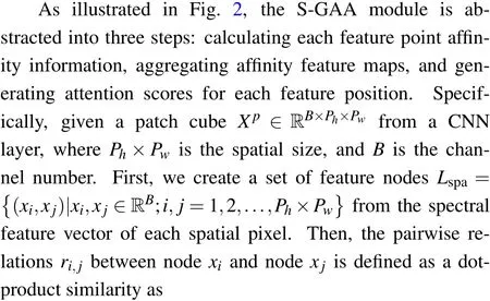
(ii)To reduce the impact of interference pixels on classification performance, a global affinity attention (GAA) module is introduced to extract the affinity relationship between each feature node from the global scope of the feature map.Specifically, this attention module has two independent feature enhancement paths: spatial global affinity attention module(S-GAA)and channel global affinity attention module(CGAA).The results show that the spatial and spectral information recalibrated by the GAA module can effectively mitigate the effects of interfering pixels and improve the classification results.

(iii) A series of experiments verify the effectiveness of the proposed network, and the classification results with ten comparison methods on three challenging HSI datasets(i.e., IP, PU, and SA) are reported. For reproducibility, the code of the proposed network will be available at https://github.com/HaiZhu-Pan/LTGCN.

The remainder of this paper is structured as follows.Some closely related works are reviewed in Section 2,including the 3D Gabor filter and CNN.In Section 3, our proposed network is presented in three parts. In Section 4,comparative experiments and ablation analysis are performed to demonstrate the effectiveness of the proposed network. Finally,Section 5 provides some concluding remarks and suggestions for future work.

2. Related works

2.1. 3D gabor filters

Hubelet al.argued that the initial layer of visual processing in the human visual system is responsible for perceiving low-level visual information.[40]The 2D Gabor filter performs well in detecting low-level texture representations and distinguishing spatial connections. It has received a great deal of attention in disciplines such as human emotional recognition[41]and texture segmentation,[42]and person re-identification.[43]In terms of HSI feature extraction, it has been extended into 3D formation to reveal the joint spatial-spectral correlations of the HSI. The 3D Gabor filter is a sinusoidal wave modulated by a 3D Gaussian function. Concretely,for a 3D Gabor function,Gis defined as follows:

where(x,y,z)denotes non-rotated spatial-spectral coordinate,(x′,y′,z′)T=R×(x,y,z)Tdenotes the rotated spatial-spectral coordinate of the 3D Gaussian envelope;Ris a rotation matrix,which is defined as Eq.(3);i denotes the imaginary units;λdenotes the wavelength of the Gabor filter;θdenotes the orientation of the normal to the parallel stripes of the Gabor function;ψdenotes the phase offset;γdenotes the ellipticity of the support of the Gabor function;σdenotes the standard deviation of the Gaussian envelope.

2.2. Convolutional neural networks

In recent years, CNNs have been successfully employed in computer vision, such as image classification,[44]object detection,[45]super-resolution,[46]and so on. Since its learning ability is significantly better than the traditional ML methods,it has become one of the most effective tools for HSI classification. Some basic convolution layers used in the proposed network are briefly described in the following.

(i)Convolutional layer: The convolutional(Conv)layers are the fundamental component of CNN.It carries the majority of the computational burden on the network. This layer performs dot product operations between the two core matrices.One matrix is a collection of learnable parameters, generally referred to as the kernel (weights). The other matrix is the limited portion of the receptive field. The convolutional layer uses different kernels to perform elemental dot product on the input image. The kernel is spatially smaller than the input image but is deeper.This implies that if the input image has three(RGB)channels,the kernel height and width will be spatially minimal, but the depth will span all three channels. In this layer,the output of a single neuron for inputxis calculated as follows:

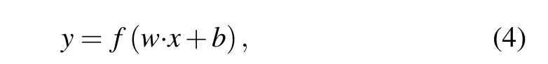
wherewandbare the filter weight and bias parameters,which are randomly initialized.f(·)denotes the nonlinear activation function.

(ii) Batch normalization layer: The batch normalization(BN) is proposed to avoid gradient vanishing and reduce the covariate shift. It normalizes the distribution of each input feature map in each layer across each minibatch to Gaussian distribution with the mean of zero and the variance of one.Furthermore, it regularizes and speeds the training process in each Conv layer, even with higher learning rates. For a layer withn-dimensional inputx=(x(1),...,x(n)), we will normalize each dimensionx(d)by the following formula:

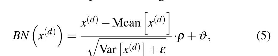
whereρandϑare denoted as learnable parameter vectors,respectively, andεis denoted as a parameter for numerical stability.

(iii)Nonlinearity layer: This layer applies a nonlinear activation function on each feature map to learn nonlinear representations. The rectified linear units(ReLu)is applied in our proposed network,which thresholds the negative value as zero and makes the positive value remain unchanged. The ReLu formula is denoted as follows:

(iv) Fully connected layer: Typically, the last part of the network comprises several fully connected layers. Each neuron node of this layer is connected with all neuron nodes of the previous layer. This layer plays the role of mapping the learned feature representation to the classifier. In order words,it integrates all the previous layers extract features and sends them to the final classifier. The parameters of this layer can account for about 80%of the whole network parameters.

(v) Dropout layer: This layer is adopted to prevent the overfitting problem of the network. Some neurons in the hidden layer are randomly ignored during the training process,thus easing the complex co-adaptation relationship between neurons.

3. Methodology

3.1. Learnable 3D gabor filter

Typically, to generate a set of 3D Gabor convolutional kernel(3D GCK)with different parameters,we embed all five fundamental parametersΓ=(λ,θ,ψ,γ,σ) in the 3D GCK construction process. Specifically, let 2k+1(k ∈N+) denote the kernel size; we setx=[−k,−k+1,...,k −1,k],y=[−k,−k+1,...,k −1,k], andz= [−k,−k+1,...,k −1,k],and then the generated 3D GCK is illustrated in Fig.1.

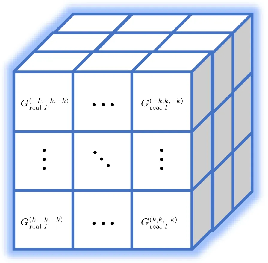
Fig.1. The 3D GCK with learnable parameters.

Different from the 3D RCK,all elements in the 3D GCK are generated from Eq. (2), where the parameters have specific meanings and are associated with each other. However,the elements in 3D RCK are randomly generated and are not associated with each other. Thus, this is the essential difference between the two convolution kernels. Additionally, the number of 3D GCK parameters is substantially reduced due to this layer has only five parameters to learn no matter how the convolution kernel size changes,whereas a 3D RCK will have(2k+1)3parameters to learn. For example, whenk=1, the number of free parameters of a 3D GCK and a 3D RCK are 5 and 27,respectively. Thus,the learning parameters of the network can be significantly reduced when the convolution kernel size becomes larger. In the BP process, only five parametersΓ=(λ,θ,ψ,γ,σ)needs to be updated through the chain rule.The gradient ofΓcan be denoted as

where every element denotes the gradient with respect to the parameter. From the above equation, it can be seen that we simply need to calculate the partial derivative of each parameter using the chain rule. TakeλandGreΓin Eq. (2), as an example,we have

A similar process can be used to derive the remaining four parameters. The above formulas demonstrate how to compute the gradient manually. In our experiments,the high-level neural networks API,such as PyTorch,is adopted to calculate the gradients automatically.

3.2. Global affinity attention module

To extract global affinity information from the feature maps, inspired by the recently published attention mechanism,[47]we design the GAA module for the proposed network. The GAA module comprises two sub-modules: SGAA and C-GAA.A detailed description of the two attention modules is given in the following texts.

3.2.1. Spatial-wise global affinity attention module

3.2.2. Channel-wise global affinity attention module

We apply a similar strategy to design the C-GAA module, which aims to analyze the weight of the various channels and recalibrate them. Figure 3 shows the architecture of the C-GAA module. The critical distinction between the two attention modules is that the pair relations are calculated channel-wise rather than spatial-wise. Thus, in what follows,we briefly overview the fundamental learning process of the C-GAA module.spe

Fig.2. Flowchart of the spatial-wise global affinity attention module.

Fig.3. Flowchart of the channel-wise global affinity attention module.

3.3. Proposed network architecture

To intuitively understand the proposed network, figure 4 shows the network architecture map using the IP dataset.It can be seen that the HSI is a 3D data cube. We denote the input HSI data asH ∈RD×M×N, whereD,M,andNrepresent the number of spectral bands and the height and width of the spatial dimensions,respectively. First,the raw HSI data are standardized to the range of 0 to 1 to make the network operation more stable. Then,the PCA is used to reduce the dimensions along with the spectral bands due to the raw HSI data containing hundreds of redundant spectral bands, during which the spatial dimension remains unchanged. Next, to perform the pixel-wise HSI classification with CNNs, the HSI data cube processed by PCA is divided into a set of 3D patch cubes centered on the labeled pixels as the network’s input. The size of input patch cubes isB×Ph×Pw, whereBdenotes the spectral band number andPh×Pwdenotes the spatial size. After that, all patch cubes are randomly divided into three collections sets, including training, validation, and testing sets. We use the training set to configure the proposed network and its hyperparameters and test the trained network on the validation set to find the best-trained network model. Then, the besttrained network model is applied to obtain evaluation metrics by testing set. Finally,all pixels except the background are fed into the network to obtain the final classification map.

Table 1. The implementation details of the proposed network on the IP datasets.

Fig.4. The architecture map of the proposed network.

In terms of the network architecture, the proposed network mainly consists of three blocks. The first is the spatialspectral block. It comprises three custom 3D GCLs. Empirically,the dimension of the 3D GCK is 5×5×5,which means that the kernel size is 5×5 in the spatial dimension and 5 in the depth dimension. Moreover, the number of convolution kernels (filters) is 8, 16, and 32, respectively, in the subsequent first,second,and third convolution layers. As the number of kernels increases, it can fully use the scalable capability of 3D Gabor filters to extract spatial-spectral information with varying scale and orientation robustness enhancement in the learning phase. Following that,the collected features from this block are fed into the GAA module with spatial and spectral attention (see Subsection 3.2) to emphasize the informative features in the feature map and suppress unnecessary ones.Generally speaking,it is difficult to achieve sufficient spatialspectral information using shallow 3D convolution operations,while using more layers of 3D convolution operations tends to increase the computational complexity. The second spatial block is connected behind the GAA module to alleviate this problem, consisting of two 2D convolution layers. The dimension of the 2D convolution kernel is 3×3,and the number of convolution kernels is 64 and 128 in the subsequent first and second convolution layers,respectively. Furthermore,the GAA module is also added after each 2D convolution operation. Next,by flattening the output of the preceding block,all of the neurons are linked to the neurons of the classification block. This block utilizes three fully connected(FC)layers to classify. The number of nodes in the last FC layer is the same as the number of classes.The number of nodes in this layer for the IP dataset is 16. Finally,the classification map is obtained.It is noted that the BN and ReLu are adopted after each convolution layer and the first two FC layers. At the same time,the dropout layer is also used after the first two FC layers to avoid overfitting. The implementation details of the proposed network on the IP datasets are listed in Table 1.

4. Experiments and discussion

In this section, three publicly available real-world HSI datasets(i.e.,IP,PU,and SA)are used to assess the feasibility and effectiveness of the proposed network. In addition, three metrics are used to quantify the model classification performance,including the overall accuracy(OA),average accuracy(AA),and kappa coefficient(k).OA is the ratio of correctly labeled samples to the total number of labeled samples in the test samples. AA is the average of all different labeled class classification accuracy.Thekis the consistency index between the classification result map and the ground truth map. All experiments are performed on a deep learning workstation with 2×Intel Xeon E5-2680 v4 @ 2.40 GHz CPU, 128 GB of RAM,8×NVIDIA 2080Ti GPUs,and the deep learning framework is PyTorch.

4.1. Hyperspectral datasets description

4.1.1. IP dataset

The first hyperspectral dataset was acquired by the airborne visible/infrared imaging spectrometer (AVIRIS) sensor over the agricultural area of North-western Indiana in June 1992,which consists of 145×145 spatial pixels and as many as 224 spectral bands. The spatial resolution of this dataset is 20-m per pixel, and the spectral resolution is 10-nm ranging from 0.4 µm to 2.5 µm. Before classification, 20 spectral bands(i.e.,104th–108th,150th–163th,and 200th)are removed from the data due to noise and water absorption. After that, the remaining 200 spectral bands are preserved for classification in this paper. The dataset has 10249 labeled samples from 16 different ground-truth classes. Most of them are various types of crops[see Fig.5]. The samples number for each class are exhaustively provided in Table 2.

Table 2. Land cover classes with the number of samples for the IP dataset.

Fig.5. (a)False-color map,(b)ground-truth map,and(c)labels of the IP dataset.

4.1.2. PU dataset

The second dataset was collected by the reflective optics system imaging spectrometer (ROSIS) sensor over the University campus at Pavia, Northern Italy, in 2003. It contains 115 spectral bands, with a resolution of 4 nm ranging from 0.43µm to 0.86µm,of which 12 bad spectral bands are commonly discarded. After discarding, the remaining 103 bands are kept for classification in this article. The spatial size of the dataset is 610×340, and the spatial resolution of 1.3-m per pixel. The ground truth consists of 9 urban land-cover types with 42776 labeled samples[see Fig.6]. The number of samples for each class is listed in Table 3.

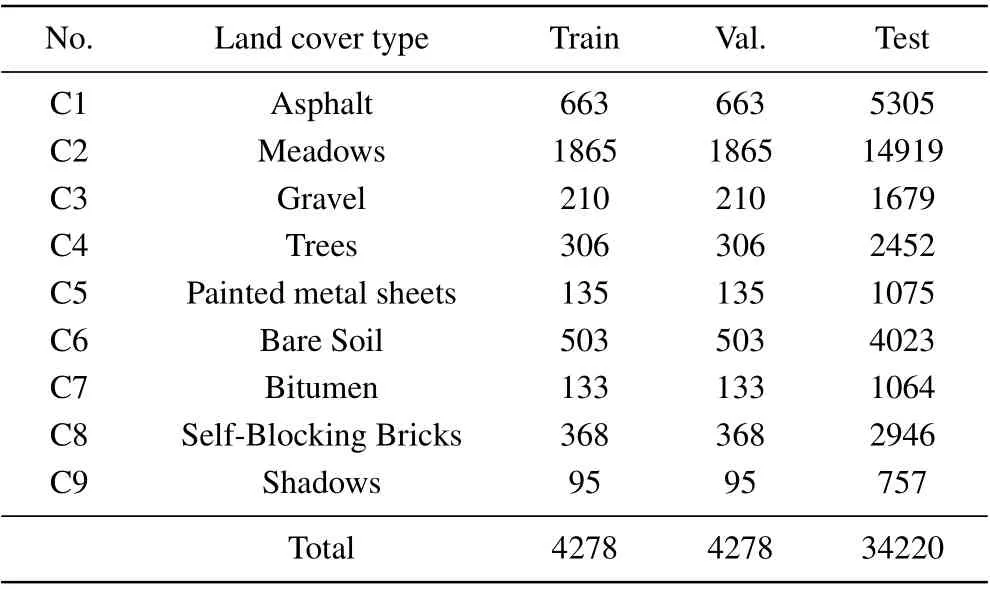
Table 3. Land cover classes with the number of samples for the PU dataset.

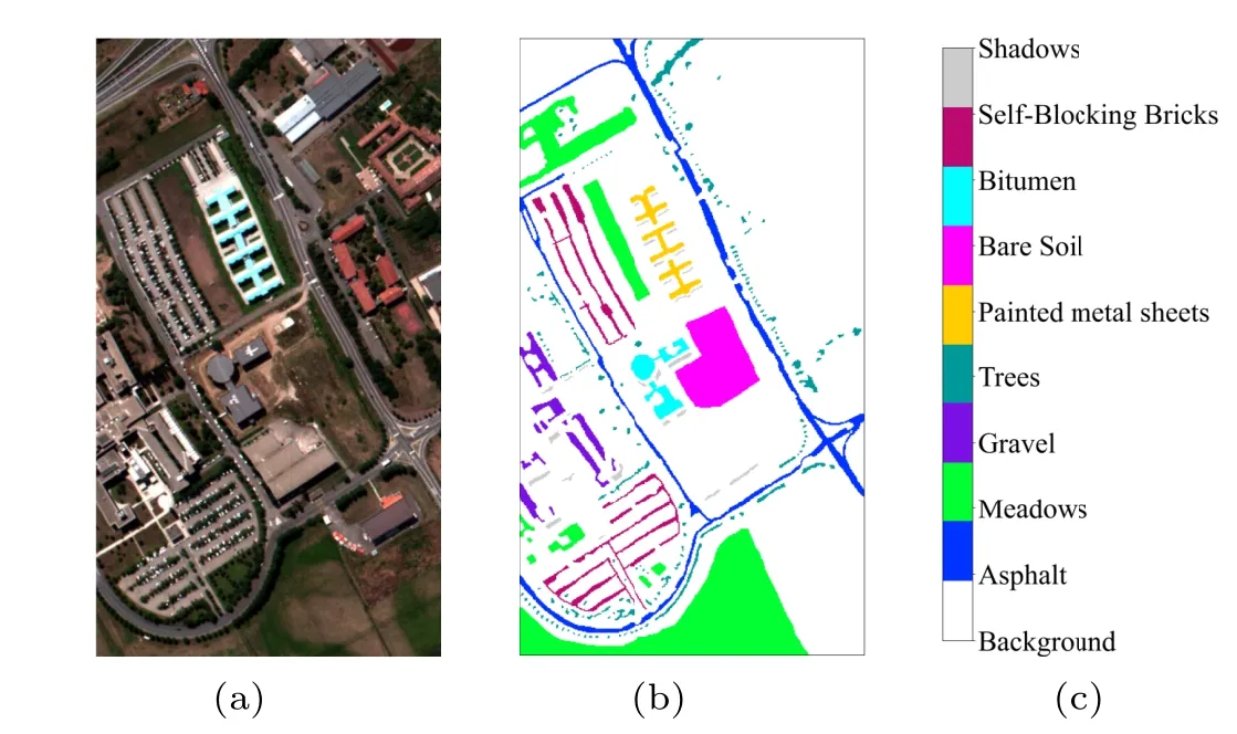
Fig.6. (a)False-colour map,(b)ground-truth map,and(c)labels of the PU dataset.

4.1.3. SA dataset

The third dataset was gathered by the AVIRIS sensor over the area of Salinas scene, California. The spatial size of the dataset is 512×217, and the spatial resolution is 18-m per pixel.It has 224 spectral bands with wavelengths ranging from 0.4µm to 2.5µm. This dataset is similar to IP.Twenty water absorption bands(i.e.,108th–112th,154th–167th,and 224th)are discarded. Subsequently,204 out of the 224 bands are reserved in this paper. There are 54129 labeled samples in total,and 16 classes of land covers are considered[see Fig.7]. The class name and the sample size are listed in Table 4.

Three hyperspectral datasets have different sizes of labeled samples and resolution,which can better verify the universality of the proposed network. There are 10249 and 42776 labeled samples for the IP and PU datasets.In contrast,the SA dataset has 54129 labeled samples. Compared with the previous two datasets,the latter has a relatively massive number of labeled samples and a more regular ground truth distribution.

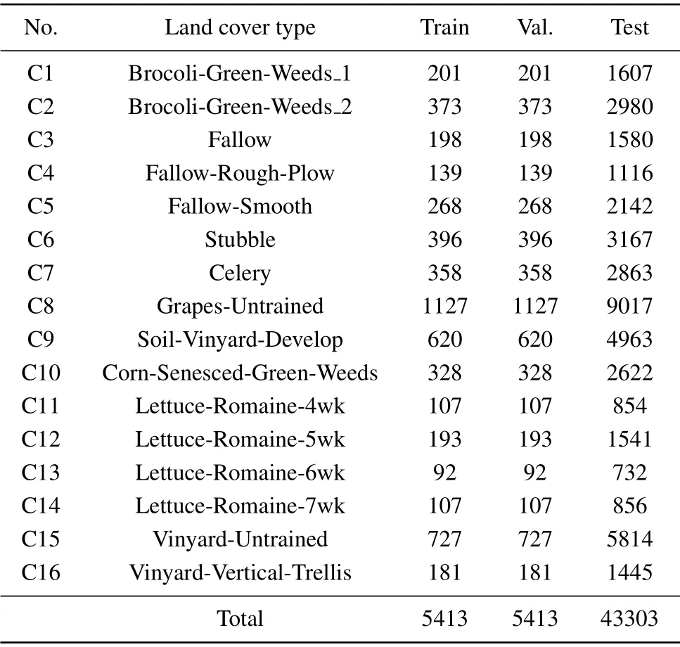
Table 4. Land cover classes with the number of samples for the SA dataset.

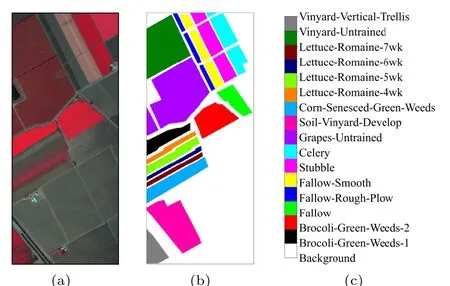
Fig.7. (a)False-colour map,(b)ground-truth map,and(c)labels of the SA dataset.

4.2. Experimental setting

To effectively illustrate and verify the effectiveness of our proposed network, four classical ML-based and six state-ofthe-art DL-based methods were utilized in our comparison.All these methods are explained as follows.

(i) Support vector machine with radial basis function(RBF-SVM): The RBF-SVM is used as a supervised classifier for original HSI data without feature extraction and dimensionality reduction.The penalty parameter C and the RBF kernel widthσare selected by five-fold cross-validation,both in the range of(10−2,102).[48]

(ii) K-nearest neighbour (KNN): The k-NN classifier is applied to the raw HSI data. The parameter of the number of neighbors in k-NN is set to be 5.

(iii)Support vector machine with 2D Gabor filters(2DGSVM):The 2D Gabor filter groups are generated by one fixed frequency of 0.5 Hz and four orientations (0◦, 45◦, 90◦, and 135◦) with the kernel size of 11×11. Then, these 2D Gabor filters are applied to extract the spatial texture features of the original HSI data. After that, these extracted spatial features as the input of the SVM classifier for classification.[14]

(iv)Support vector machine with 3D Gabor filters(3DGSVM): Latest research in Ref. [17] shows that the 3D Gabor filter parallel to the spectral direction can adopt more identifying information than other orientations. Thus, only one 3D Gabor filter with a frequency 0.5 Hz is directly convolved with the raw HSI data cube to extract spatial-spectral features as input for the SVM classifier in our experiments.

(v)2D CNN:2D convolution kernels are used in CNNs,called the spatial-based classification approach.[21]The network mainly includes four 1×1 2D convolution layers, two normalization layers, two drop layers, and one average pooling layer. In addition, the model removes the FC layers to reduce the number of trainable parameters.

(vi)3D CNN:3D convolution kernels are used in CNNs,which can directly extract the spatial-spectral feature of the HSI cube without relying on any pre-processing.[49]It is constructed with two 3D convolution layers and a logistic regression layer. A max-pooling layer follows each convolution layer.

(vii) 3D–2D CNN: To extract more discriminative features, 2D CNN and 3D CNN are used together in HSI classification to fully utilize the spatial-spectral features.[24]The hybrid CNN model has three 3D convolution layers, two 2D convolution layers,and two fully connected layers. Each convolution layer is followed by a bath normalization (BN) and an activation layer.

(viii)2D–3D multibranch CNN(MB-CNN):Three CNN branches fusion networks are applied to extract deep-level features. Each branch has a different kernel size. This model first uses PCA to reduce the spectral dimension of raw HSI data before input. After that, they extracted spatial-spectral joint features through a three-branch network. Finally,four FC layers and a SoftMax layer for classification.[25]

(ix)2D Gabor CNN(2DG-CNN):In this model,PCA is also used on the spectral domain to reduce computation cost and applied Gabor filters to extract the edge and texture feature of HSI as the network input.[27]The network architecture consists of one convolution layer with BN,ReLu,and dropout.At the end of the model, SoftMax is applied to conclude the classification result.

(x) Attention CNN (Atten-CNN): The learnable spectral attention model is inserted into a 2D CNN between the input and the first convolution layer. It is constructed with three 2D convolution blocks with max-pooling and two FC layers.In 2D CNN blocks, convolution layers are followed by a BN layer and a ReLu activation function.[33]

For the comparison to be meaningful and fair,the training set of the proposed method and compared methods adopt the same experimental setup, including pre-processing steps and hyperparameter setup. In the proposed network, the Adam(adaptive motion estimation) optimizer is used to update the parameters.The learning rate and weight decay of the network are set to 0.001, respectively. The learning rate is divided by 2 for every 20 training epochs,which can save computational cost and reduce manual adjustment of the learning rate. The number of training epochs is set to 100, and the batch size is set to 128.The dropout with a drop rate of 0.4 is used in the FC layer. To avoid any bias of random factors,all experiments are randomly repeated in ten trials. The mean values and variance of each metric(i.e.,OA,AA,andk)are reported.

4.3. Comparison with other methods

In this subsection,to demonstrate the effectiveness of the proposed network, ten comparison methods, including four classical ML-based methods and six state-of-the-are DL-based methods,are used on three different scene datasets. Moreover,the classification results of the proposed network are reported quantitatively and visually.

First, we quantitatively evaluate the performance of the proposed network and the other comparative methods in Table 4 on the IP dataset. As can be observed from Table 4,the proposed network acquired competitive results compared to the other comparison methods on three metrics. Specifically,the Gabor-based methods have higher accuracy than the RBF-SVM or KNN methods.The difference is that the former uses Gabor filters to extract prior knowledge before the classification, while the latter does not. It can be seen that the Gabor features have a significant improvement in classification performance. Compared with those DL-based methods, the proposed network achieves competitive results. In particular,from Table 5,it is clear that our proposed network delivers the best OA (98.3%), AA (96.3%), andk(0.98). It achieves the accuracy of 7.8%, 2.8%, 4.7%, 3.7%, 3.2%, and 7.1% more than 2D CNN,3D CNN,3D–2D CNN,MB-CNN,2DG-CNN,and Atten-CNN,respectively.Because the deep networks have an inherent hierarchical structure,which can automatically extract deep-level information from the HSI data. Therefore,these DL-based methods are commonly superior to classic ML-based methods. By comparing the Atten-CNN with 2D CNN, it can be seen that the attention module improves the OA of 2D CNN by 0.7%, the AA of 2D CNN by 0.4%, and thekof 2D CNN by 0.1, which could be attributed to the spectral-attention module contribution. Besides, since introduced global attention modules utilize both spatial-spectral information and global scope relation of HSI,the classification accuracies obtained by the proposed network are higher than Atten-CNN.

Table 5. Classification results of different methods on the IP dataset.

Fig.8. (a)Ground-truth map and classification maps on the IP dataset by(b)RBF-SVM,(c)KNN,(d)2DG-SVM,(e)3DG-SVM,(f)2D CNN,(g)3D CNN,(h)3D–2D CNN,(i)MB-CNN,(j)2DG-CNN,(k)Atten-CNN,(l)proposed.

Table 6. Classification results of different methods on the PU dataset..

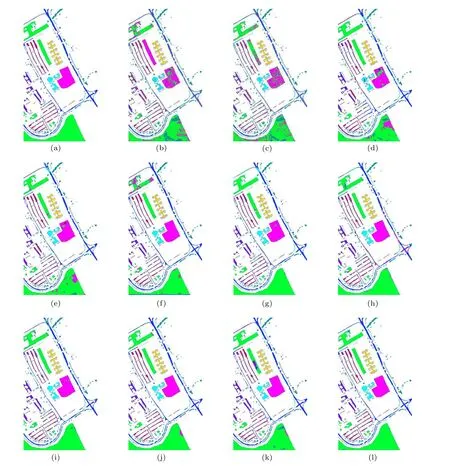
Fig. 9. (a) Ground-truth map and classification maps on the PU dataset by (b) RBF-SVM, (c) KNN, (d) 2DG-SVM, (e) 3DG-SVM, (f) 2D CNN, (g) 3D CNN,(h)3D–2D CNN,(i)MB-CNN,(j)2DG-CNN,(k)Atten-CNN,(l)proposed.

Figure 8 depicts the ground truth map and classification maps of multiple methods in a single experiment on the IP dataset. Unlike other methods, less salt-and-pepper noise is shown in the proposed network classification map[see Fig.8(l)]. As shown in Fig.8,the classification map obtained by Gabor-based CNN is smoother than those obtained from other methods. In contrast,the classification map of the RBFSVM [see Fig. 8(b)] and KNN [see Fig. 8(c)] methods, they have much salt-and-pepper noise. Meanwhile, it can be seen from the area marked by the red box in Fig. 8, our proposed method is more accurate for small ground objects compared to other comparison methods [see Figs. 8(b)–8(k)]. This is mainly owing to the inclusion of the global attention module in our proposed network, which could extract more discriminative global features from tiny ground objects while successfully mitigating the impacts of interfering pixels. Moreover,from Fig.8, it can be noted that the classification map of our proposed network has more consistent with the ground-truth map than other methods. All observations confirm that the learned 3D GCK and GAA modules play a positive role in the proposed network.

Second, the detailed classification results on the PU dataset are listed in Table 6.Compared to the previous dataset,the spatial resolution of this dataset is large(1.3-m per pixel),so the classification accuracy of all ML-based methods is improved. For DL-based methods, the classification accuracy fluctuates in a narrow range due to changes in the dataset,yet our proposed network still presents the highest accuracy in most categories. Specifically, our proposed network achieves maximum OA(98.9%),AA(99.1%),andk(0.99)with minimum standard deviation, which indicates the proposed methods have strong stability in a different dataset. It delivers overall accuracy 26.6%, 23.6%,19.2%, 9.5%, 8.2%, 5.4%, 6.9%,5.5%, 4.7%, and 5.3% more than RBF-SVM, KNN, 2DGSVM,3DG-SVM,2D CNN,3D CNN,MB-CNN,2DG-CNN,and Atten-CNN, respectively. Among the above-mentioned methods, RBF-SVM acquires not too high classification accuracies since it does not use any feature extraction strategy before classification. Additionally, we can see that the Gabor-based methods outperform the other ML-based method in terms of accuracy,which indicate the efficiency of the Gabor feature for the HSI classification. For further visually,the ground-truth map and the predicted maps obtained by different methods in a single experiment at PU are provided in Fig.9. It should be mentioned that the four classification maps acquired by the four Gabor-based methods [see Figs. 9(d), 9(e), 9(g),and 9(l)] display smooth shapes in some categories (such as the categories in C2 and C6). This phenomenon is mostly owing to the Gabor filters fusion technique. These observations indicate that the proposed network can deal with complicated urban situations.

Finally, in Table 7, we exhibit the classification accuracies and three metrics of the proposed network and comparative methods on the SA dataset. It is worth noting that almost all methods significantly improve classification accuracy.That is mainly due to the uniform distribution of ground objects on the Salinas dataset, making classification easier. Nevertheless, the RBF-SVM still provides the worst prediction result. In terms of classification accuracy,the proposed network is 18.4%better than RBF-SVM,17.7 better than KNN,9.3%better than 2DG-SVM,8.6%better than 3DG-SVM,7.3%better than 2D CNN,4.1%better than 3D CNN,5.2%better than 3D–2D CNN, 4.8% better than MB-CNN, 2.9% better than 2DG-CNN, and 4.6% better than Atten-CNN. Similarly, the classification maps of the ten compared methods are shown in Fig. 6, and a similar conclusion can be concluded as with the PU dataset. Moreover,it can be easily observed that from Figs.6(b)–6(k),the presence of two categories in this dataset(i.e.,C8 and C15),which are harder to classify and have lower accuracy than other categories. This is mainly due to the very similar texture and spectral bands between C8 and C15. The two categories of objects can be precisely distinguished and classified in our proposed network due to the specially designed GAA module and learnable 3D GCK.

Fig.10. (a)Ground-truth map and classification maps on the SA dataset by(b)RBF-SVM,(c)KNN,(d)2DG-SVM,(e)3DG-SVM,(f)2D CNN,(g)3D CNN,(h)3D–2D CNN,(i)MB-CNN,(j)2DG-CNN,(k)Atten-CNN,and(l)proposed.

4.4. Impact of training proportion

In this subsection,we use a different proportion of training samples to verify the effectiveness and robustness of the proposed network. Specifically,the training samples for each dataset are randomly selected from all samples, five different proportions (i.e., 1%, 3%, 5%, 7%, 9%) of training samples are selected for each category,and the rest are used as testing samples. The OA,AA,andkmetrics for the different methods on the three datasets are shown in Figs.11–13. As can be observed from the three sets of figures,when compared to other approaches, our proposed network consistently maintains the most significant classification accuracy in various proportions of training data. Furthermore,Table 8 shows the classification results of the proposed network for three datasets with different training samples. From Table 8, it can be seen that the OA of the proposed method increases with the increased proportion of the training samples. It is indicated that the more the proportion of training samples, the higher the proportion of correctly classified samples in the overall test sample. In terms of AA,a similar conclusion can be obtained as with OA.Next,thekof our proposed network is almost between 0.9 and 1 on three datasets,which is higher than other methods in most cases,and thus,our proposed method presents a better degree of classification consistency.In conclusion,many experiments show that our proposed network has the same excellent classification performance under the variation of training samples.

Table 8. Classification results of the proposed network for three datasets with different training samples.

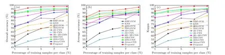
Fig.11. Classification accuracy based on different percentages of training samples on the IP dataset: (a)OA(%),(b)AA(%),(c)k.

Fig.12. Classification accuracy based on different percentages of training samples on the PU dataset: (a)OA(%),(b)AA(%),(c)k.

Fig.13. Classification accuracy based on different percentages of training samples on the SA dataset: (a)OA(%),(b)AA(%),(c)k.

4.5. Impact of patch size

In this subsection,we explore the effect between the patch size and the classification accuracy of the proposed network.In general, if the patch size of the input cube is too small, it will not be enough to contain rich spatial features.It will cause some helpful features to be lost,and the classification performance will also be decreased. On the other hand,if the patch size of the input cube is too large,it will contain more mixed pixels and increase the computation cost. Therefore, an appropriate patch size should be determined by the classification accuracy. Figure 14 depicts the classification accuracy with different patch sizes ranging from 11 to 31 with a 2-pixel interval. According to Figs. 14(a) and 14(c), with the increase of the patch size,the classification accuracy of the IP and SA datasets gradually increases, and the best classification accuracy is acquired when the patch size is 25×25. However,the best classification accuracy for the PU dataset is obtained when the patch size is 21×21[see Fig.14(b)]. The patch size of the PU dataset is slightly reduced compared to the former two datasets. It is mainly because so many complex and variable urban scenes are included in the PU that the patch size is reduced. In conclusion, we use 25×25 as the patch size on the IP and SA datasets and use 21×21 on the PU dataset in the experiments.

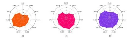
Fig.14. Visualization of the classification accuracy with different patch sizes on three datasets: (a)IP,(b)PU,and(c)SA.

4.6. Ablation analysis toward the global affinity attention module

In this subsection,we perform the ablation analysis of the GAA module on three datasets. To ensure a fair comparison,all ablation experiments are trained using the identical training settings as described in Subsection 3.3. The classification accuracy is reported in Table 9. In Table 9,baseline represents that the GAA is not used in the proposed network, S-GAA and C-GAA represent that only spatial and channel GAA are used in the proposed network, respectively, and GAA represents that both spatial and channel GAA are used in the proposed network. According to the results,we can observe that no matter S-GAA or C-GAA effectively improves the classification accuracy over the baseline. It is worthwhile to note that even though the classification accuracy of the Baseline is already very high on the SA dataset, the S-GAA, C-GAA,and GAA improve the OA by 2.1%,2.7%,and 3.1%,respectively. More visually, the classification maps of the ablation experiments on the three datasets are shown in Figs. 15–17.Experiment results consistently show that compared to using the S-GAA module alone or the C-GAA module alone, the GAA module can learn more discriminative features and increase the classification accuracy.

Table 9. Ablation analysis toward the global affinity attention module of the proposed network on different datasets.

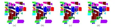
Fig.15. Classification results of ablation experiments on the IP dataset: (a)baseline,(b)S-GAA,(c)C-GAA,(d)GAA.

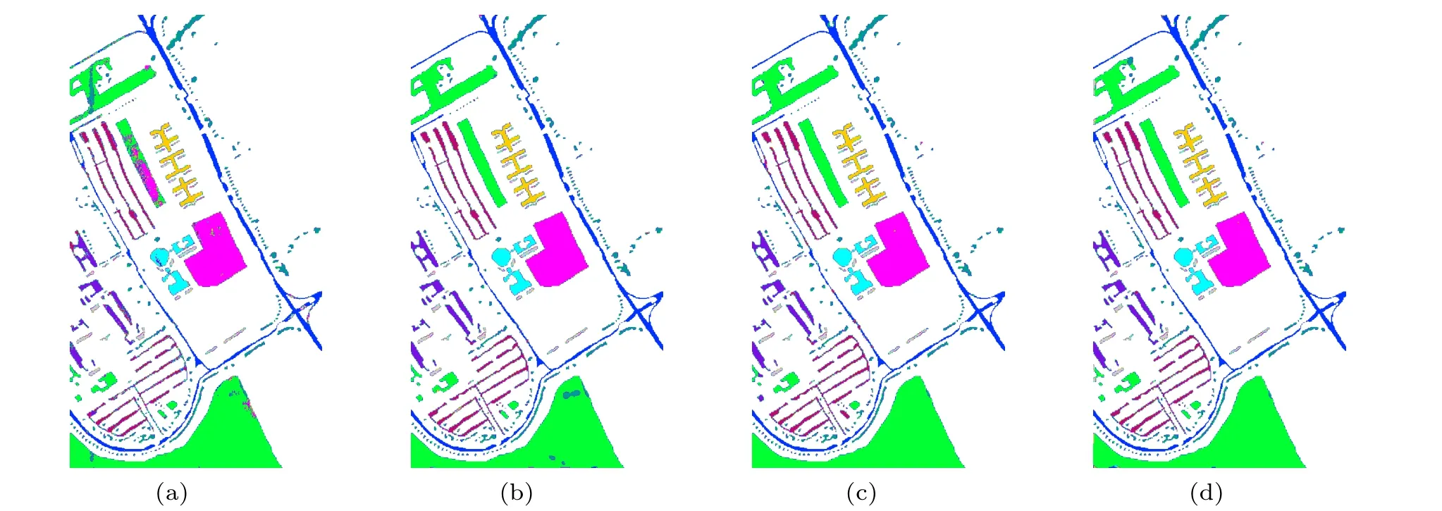
Fig.16. Classification results of ablation experiments on the PU dataset: (a)baseline,(b)S-GAA,(c)C-GAA,(d)GAA.

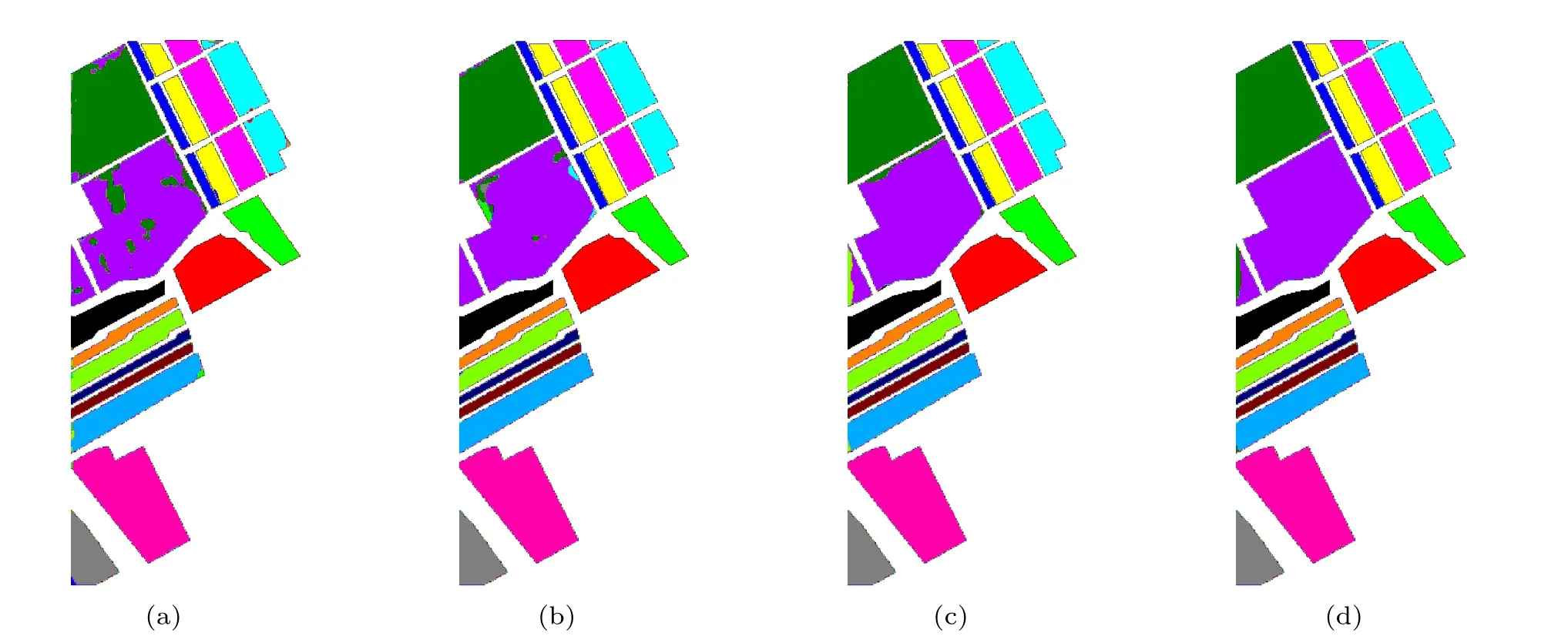
Fig.17. Classification results of ablation experiments on the SA dataset: (a)baseline,(b)S-GAA,(c)C-GAA,(d)GAA.

5. Conclusions

In this paper,we proposed a learnable 3D Gabor convolutional network with global affinity attention for HSI classification. In the spatial-spectral block, we combine the 3D Gabor filter with CNN, in which the 3D RCL is replaced by the 3D GCL.Therefore,the proposed network not only makes full use of the powerful learning ability of CNNs but also has the characteristics of 3D Gabor filters. In addition, to balance model efficacy against efficiency,we use 2D CNN to fuse the feature maps extracted by 3D GCL. The GAA module is introduced in the proposed network,which can mine more discriminative features from the global scope of each feature point and mitigate the impact of the interference pixels on the classification performance.

In terms of the experiment, four ML-based methods and six DL-based methods are conducted as compared methods.Three real-world HSI datasets are used to evaluate the classification performance of the proposed network,including IP,PU,and SA. It can be seen from the experimental result that our proposed network achieves an outstanding classification performance than other state-of-the-art methods. Extensive ablation experiments verify the rationality of the GAA module of the proposed network. In our future work,we will explore new types of 3D filters that may be applied to the convolution layer, which provides a realistic future research route for the CNN-based HSI classification.

Acknowledgments

Project supported by the Fundamental Research Funds in Heilongjiang Provincial Universities (Grant No. 145109218)and the Natural Science Foundation of Heilongjiang Province of China(Grant No.LH2020F050).