Chen MA and Tim LI

1 Jiangsu Meteorological Observatory, Jiangsu Meteorological Bureau, Nanjing 210019, China

2 Key Laboratory of Meteorological Disaster, Ministry of Education (KLME)/Joint International Research Laboratory of Climate and Environmental Change (ILCEC)/Collaborative Innovation Center on Forecast and Evaluation of Meteorological Disasters (CIC-FEMD),Nanjing University of Information Science &Technology, Nanjing 210044, China

3 International Pacific Research Center and Department of Atmospheric Sciences, School of Ocean and Earth Science and Technology, University of Hawaii, HI 96822, USA

4 Key Laboratory of Transportation Meteorology, China Meteorological Administration, Nanjing 210019, China

ABSTRACT The relative impact of environmental parameters on tropical cyclone (TC) intensification rate (IR) was investigated through a box difference index (BDI) method, using TC best track data from Joint Typhoon Warning Center and environmental fields from the NCEP final analysis data over the western North Pacific (WNP) during 2000–2018.There are total 6307 TC samples with a 6-h interval, of which about 14% belong to rapid intensification (RI) category. The analysis shows that RI occurs more frequently with higher environmental sea surface temperature, higher oceanic heat content, and lower upper-tropospheric temperature. A moderate easterly shear is more favorable for TC intensification. TC intensification happens mostly equatorward of 20°N while TC weakening happens mostly when TCs are located in the northwest of the basin. Mid-tropospheric relative humidity and vertical velocity are good indicators separating the intensification and non-intensification groups. A statistical model for TC intensity prediction was constructed based on six environmental predictors, with or without initial TC intensity. Both models are skillful based on Brier skill score (BSS) relative to climatology and in comparison with other statistical models, for both a training period (2000–2018) and an independent forecast period (2019–2020).

Key words: tropical cyclone, rapid intensification, prediction model

1. Introduction

Rapid intensification (RI) is common in most of intense tropical cyclones (TCs), as about 70 and 83 percent of super typhoons underwent RI at least once during their lifetime in the western North Pacific (WNP) and North Atlantic, respectively (Kaplan and DeMaria, 2003;Shu et al., 2012). Before the TC makes landfall, the sudden and rapid intensification will bring serious uncertainty to the safety of life and property along the coast.As the global warming intensifies, TCs may intensify much more rapidly before hitting land, making hurricane forecasting even more challenging (Emanuel, 2017). Although the ability of operational forecasting models to predict the TC track has increased substantially, the improvement in the TC intensity forecasting is less (De-Maria et al., 2014; Emanuel and Zhang, 2016; Tallapragada et al., 2016). In particular, the operational prediction of RI is much more difficult (Titley and Elsberry,2000; Elsberry et al., 2007; Knaff et al., 2018; DeMaria et al., 2021).

The intensity change of TC depends on many environmental factors. Kaplan and DeMaria (2003) identified general synoptic conditions conducive to RI, including weak vertical shear, high low-level relative humidity,warm sea surface temperature (SST), strong upper-level easterly wind, and some external forcing such as trough systems. In addition, the oceanic heat content (OHC),which is a variable to measure the heat and depth of warm water available for TCs, has been shown to be a better predictor for RI than the SST alone (Wada and Usui, 2007; Shay and Brewster, 2010). Significant distinguishing characteristics of the TC–trough interactions were identified by Ventham and Wang (2007) for RI and non-RI scenarios in the WNP. Hanley et al. (2001) identified that a small-scale upper-level potential vorticity anomaly and TC mutually approach each other to within 500 km of the TC center just prior to the onset of RI.Their study concluded that vertical shear is the deciding factor on the TC–trough interactions. Wei et al. (2018)explored the effect of vertical wind shear with different directions on TC intensity change based on TCs over the WNP. Their result suggested that a westerly shear is not conducive to the TC intensification than easterly shear.With moderate vertical wind shear (5–10 m s-1), strong updrafts may appear in the enhanced TC circulation, resulting in a more symmetrical convective structure(Kanada and Wada, 2015; Rogers et al., 2016; Leighton et al., 2018). Dunion and Velden (2004) pointed out that the dry air in the middle and low layers weakens the intensity of TCs, so a relatively humid environment is favor to TC intensification.

Although these environmental characteristics are the most likely modes when RI occurs, which environmental variable is the most necessary condition for the occurrence of RI is still unclear. In order to predict the RI, Kaplan et al. (2010) developed a linear weighting index for the Atlantic and eastern North Pacific basin. Shu et al.(2012) applied this method on WNP basin. Lee et al.(2015) selected seven predictors and developed a multiple linear regression model for TC intensity. However,the effect of environmental variables on the TC intensification rate (IR) is nonlinear. Different from previous studies that using a linear model to estimate the probability of RI (Kaplan and DeMaria, 2003; Kaplan et al.,2010; Shu et al., 2012; Lee et al., 2015; Knaff et al.,2018), this study is dedicated to establishing a nonlinear RI probability prediction model based on the TC surrounding environment.

The rest of this paper is organized as follows. The data and methods for the study are described in Section 2, and the forecasting predictors for TC RI are selected as well.In Section 3, composites of key surrounding environments are presented to identify the environmental characteristics among different IR groups. In Section 4, the least squares method is applied to establish the probability model of TC RI based on surrounding environmental variables and the independent verification is presented as well. Finally, major findings of this study are summarized and discussed in Section 5.

2. Data and method

2.1 Data

In this study, the TC dataset is derived from Joint Typhoon Warning Center (JTWC) best-track dataset,which contains the information of TC location and intensity from 2000 to 2018 over the WNP basin at a 6-h interval. The TC surrounding environment is derived from NCEP final analysis data in a 6-h interval with a horizontal resolution of 1° × 1°. The NCEP Global Ocean Data Assimilation System (GODAS) pentad dataset is employed to calculate the OHC (Saha et al., 2006).The GODAS has a constant zonal resolution of 1° and meridional grid of 1/3°, and has 40 levels with a 10-m resolution in the upper 200 m.

2.2 Definition of IR

The maximum wind speed (MWS) of TC is chosen as the intensity metric. The selected samples in this study cover all TCs reaching the intensity of tropical storm(MWS exceeds 17 m s-1). As the time interval of JTWC dataset is 6 h, to make full use of the time resolution of the data, the IR of TC is defined as the average of 12-and 24-h intensity change rate:

where IR is the intensification rate, andVis the maximum wind speed. The IR is evaluated by using the central difference. The number of eligible samples is 6307. Figure 1 displays the probability density function of IR in WNP basin during 2000–2018. It is similar to the global probability density function during 1982–2009 (Bhatia et al.,2019). As shown in Fig. 1, 24-h intensity changes of TCs are generally normally distributed and are mainly concentrated in the interval of -20 to 20 knots. There are more intensifying cases than weakening cases, because most of the weakening cases happen when a TC approaches land but such areas are relatively small compared to the open ocean. The TC has enough time to develop over the ocean and decays quickly when it approaches land.

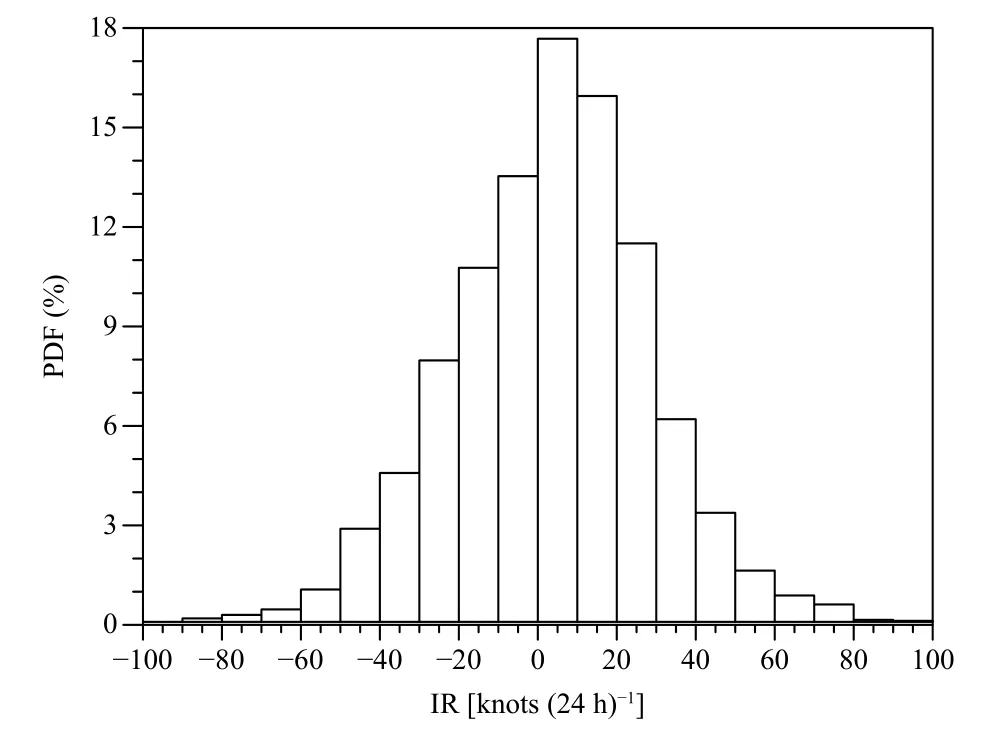
Fig. 1. Probability density function (PDF) of the intensification rates[knots (24 h)-1] for TCs in WNP during 2000-2018.

Fig. 2. Geographical distribution of five groups of IR: RI (red dots), SI (orange), N (black), SW (green), and RW (blue) in WNP from 2000 to 2018.

In Kaplan and DeMaria (2003), the RI was defined as the maximum surface wind speed increase of 30 knots over 24-h period. In this study, all cases are categorized into five groups in terms of their IR: RI [IR ≥ 30 knots(24 h)-1]; SI [slowly intensifying, 10 ≤ IR < 30 knots (24 h)-1]; N [neutral, -10 ≤ IR < 10 knots (24 h)-1]; SW[slowly weakening, -30 ≤ IR < -10 knots (24 h)-1]; and RW [rapidly weakening, IR < -30 knots (24 h)-1].Table 1 shows the number and proportion of each group of samples. From the perspective of climate statistics, the probability of TC RI over the WNP is about 13.6%.Figure 2 shows the geographic distribution of all five groups of IRs represented by different colors. Intensifying cases (SI and RI) are located mostly equatorward of 20°N and weakening cases (SW and RW) are mainly located in the northwest of intensifying cases. Neutral cases(N) are more evenly distributed among weakening and intensifying groups. As the occurrence of TC RI has a clear correlation with the TC location, we use the differ-ence between longitude and latitude (Lon - Lat) to describe this geographical distribution feature. The larger the Lon - Lat value, the more the position of the TC is to the southeast. Statistically significant differences at the 95% confidence level are found among different IR groups for the Lon - Lat.

Table 1. Categories of TC intensity change rate [knots (24 h)-1],definitions, sample sizes, and percentage for the WNP basin from 2000 to 2018

2.3 Data filtering and selection of predictors

Before further analysis, an 11-day running mean is applied to the reanalysis data to extract the low frequency environment. The selection of environmental atmospheric and oceanic variables is subjective according to factors that are well known to affect the TC intensity change. In this study, the chosen variables are SST, temperature, relative vorticity, divergence, relative humidity, specific humidity, vertical velocity, geographical distribution (Lon -Lat), OHC, vertical wind shear, and vertical zonal wind shear. Briefly, the SST, temperature, relative vorticity,divergence, relative humidity, specific humidity, and vertical velocity are calculated by the area average of corresponding low frequency fields within a range of 10° × 10°at the TC location. The Lon - Lat is the difference between the longitude and latitude of the TC center. The OHC is defined as the low-frequency sea potential temperature integrated vertically downward at a depth of 300 m within a range of 10° × 10° at the TC location. The vertical wind shear (the vertical zonal wind shear) is calculated by subtracting 850-hPa total (zonal) wind speed from 200-hPa total (zonal) wind speed, averaged within a range of 10° × 10° at the TC center.

However, not all environmental fields are critical to the TC RI. In order to figure out the key environmental variables associated with the TC RI, our strategy is carried out in two steps. First, for variables that we list above, the significancettest is employed to determine whether the difference between the RI group and other groups is significant. It is worth mentioning that TCs in the RW group are generally close to the land and terrain areas (Fig. 2). The IR in this group is mainly affected by surface land and terrain friction. Therefore, the environmental field difference between RI and RW is not considered when selecting RI predictors. Figure 3 shows the temperature profile difference between the RI group and other groups as an example. The red dot at each vertical level indicates that the temperature difference at that level is statistically significant at the 95% confidence level. It can be seen that the temperature difference between the RI and SW groups is the most obvious (Fig.3c). In addition, according to the distribution of red dots and the difference value, significant difference appears in the bottom and upper layers of the atmosphere. This result demonstrates that the more unstable atmospheric condition is favorable for the growth of the TC intensity,which makes a larger probability of RI. Notably, the differences of low-frequency environmental vorticity and divergence fields between the RI group and other groups are statistically insignificant at all vertical levels (figure omitted). This is consistent with the result of Kaplan and DeMaria (2003). They pointed out that the difference of area-averaged 850-hPa vorticity between the RI and non-RI groups is not significant. By using the method of significance test, following variables are primarily selected as key environmental variables affecting the RI: SST(TS), 200-hPa temperature (T0), 500-hPa relative humidity (RH500), 700-hPa specific humidity (SH700), 400-hPa vertical velocity (ω400), vertical zonal wind shear(VUS), vertical wind shear (VWS), OHC, and Lon - Lat.

Fig. 3. Differences (ΔT) between the low-frequency temperature composites of the RI and (a) SI, (b) N, (c) SW from 2000 to 2018 within a 10°× 10° area centered at the TC center. Red dot indicates that the difference is statistically significant at 95% confidence level.

Next, the box difference index (BDI) method is applied on the variables passing the significance test. BDI is a non-dimensional number used to describe the difference between two sets of data (Peng et al., 2012). The BDI between two groups is defined as:

whereMandσdenote the mean and standard deviation of the variable, and the subscripts “A” and “B” represent different groups of the same variable (e.g., the SST in RI and SW groups). The larger the difference between the mean and the smaller the sum of the standard deviation between two groups, the larger the BDI, and the variable is more instinctively different between two groups. Although different variables have different units, the relative importance to the TC RI can be revealed by the ranking of BDI. Figure 4 shows the BDI of key environmental variables between the RI and other groups. As bothTSandT0show large differences (Figs. 4a, b), a difference between SST and temperature at 200 hPa (TS-T0) actually has the largest BDI. This parameter reflects the atmospheric instability and is the major contributor to the TC maximum potential intensity (Emanuel, 1986; Holland, 1997). According to the ranking of BDI, six variables are chosen as TC RI predictors:TS-T0, OHC,VUS, Lon - Lat, ω400, and RH500.

3. Environment characteristics among different IR groups

In this section, composite results of six predictors for different IR groups are presented and discussed. Figure 5 shows the distributions ofTS,T0, RH500, ω400, Lon -Lat, OHC, and VUS among five groups. The solid box contains the mean and one standard deviation. There is a significant correlation between the TC IR and the surrounding SST (Fig. 5a). The higher the SST, the larger the TC IR, and the TC is more likely to have a RI process. In addition, from the perspective of the dispersion of SST, the RI phenomenon has stricter requirement on the SST, as RI is difficult to appear when the SST is low.The performance ofT0is the opposite of the SST (Fig.5b). When the temperature at 200-hPa level is low, the TC tends to occur RI. The differences ofT0among the N,SW, and RW groups are small. Specifically, the higher the SST, the lower the upper-level temperature, and the more unstable the atmosphere is, the environment is more conducive to occur RI. This is whyTS-T0is chosen as a predictor. From the result of moisture (Fig.5c), the higher the relative humidity in the middle layer,the greater the IR. However, consistent with the BDI ranking results (Fig. 4a), the distinction of relative humidity between the RI and SI groups is not obvious,which is mainly reflected in the slight difference of the mean. Although the RH500 cannot describe the environmental difference between the RI and SI, it is still a good indicator that can separate intensification cases from nonintensification cases. The ascending motion is observed in the middle level among five groups (Fig. 5d). The RI group has the strongest ascending motion. Consistent with the results in Fig. 2, although the difference between longitude and latitude cannot separate RI cases from SI cases well, it can be used to distinguish whether the TC intensity is increasing or decreasing (Fig. 5e). The TC with negative intensification rate tends to appear in the northwest of the WNP, so the value of Lon - Lat is small. According to Carnot heat engine theory, the ocean is the energy source of the TC, as the thermal energy is imported from the warm underlying ocean (Emanuel,1988). In addition, strong TC can cause the sea below to surge. The OHC is the key to maintain warm SST when the TC passes, so that the TC can continue to intensify(Shay and Brewster, 2010; Lin et al., 2021). The RI group has the highest mean OHC and the minimum standard deviation (Fig. 5f). This result is similar to the performance of SST (Fig. 5a). The TC RI requires high OHC and hardly occurs when the OHC is not high enough. Meanwhile, the RW group has the largest OHC standard deviation. This result may be due, in part, to that TCs in the RW group are generally close to terrain areas,and the ocean depth may not reach 300 m. The finding of easterly shear is more favor for the TC intensification than westerly shear is consistent with the results of Wei et al. (2018) (Fig. 5g). The strong westerly shear is not conducive to the intensification of TC.

Fig. 4. Environmental differences between RI and (a) SI, (b) N, (c)SW groups using BDI analysis for WNP TCs from 2000 to 2018. The number above the bar is the BDI value.

Fig. 5. Distributions of area-averaged environmental (a) TS (K), (b) T0 (K), (c) RH500, (d) ω400 (10-1 Pa s-1), (e) Lon - Lat, (f) OHC (K), and(g) VUS (m s-1) centered at the TC center for five IR groups. The solid box contains the mean and one standard deviation.

4. Construction of an intensity forecast model based on key environmental parameters

In Section 2, six variables (TS-T0, OHC, VUS, Lon -Lat, ω400, and RH500) are chosen as TC RI predictors by using BDI method. Here, the least squares method is employed to fit the relationship between the environmental field and the IR. A statistical model for the estimated intensification rate of TC is constructed with options considering or not considering initial TC intensity,and they are named as IRenand IRe, respectively. In the form of exponential multiplication, IReis defined as:

where coefficientsa–fcan be determined based on the least squares method. For convenience, natural logarithm will be applied at both sides of Eq. (3). Before applying logarithm operations, it is necessary to adjust the value of predictors and IR into non-dimensional numbers and ensure that they are all positive. If each term at the right-hand side of Eq. (3) (e.g., OHCb) is less than 1,the final product will be less than 1. This implies that all predictors are not conducive to the TC intensification at this time so that TC intensity will decrease. On the contrary, if each term at the right-hand side of Eq. (3) is larger than 1, TC intensity tends to increase.

Prior to applying natural logarithm to Eq. (3), a procedure is applied to make sure that the values of all nondimensional terms at both sides of Eq. (3) are positive.First, we calculate the first quartile and the third quartile for each predictor in the RI group. Next, we normalize the predictors by dividing each predictor with the first quartile. A special treatment needs to be carried out for the vertical velocity and vertical zonal wind shear as they are negative. By adding a maximum absolute value in the two terms before the normalization, we ensure that the two terms are both positive. Given the range of IR from-100 to 100 (Fig. 1), we simply normalize this left-hand side term of Eq. (3) by adding 100 to its original value and then dividing 100 so that the non-dimensional value is ranging between 0 and 2. Below are specific treatments for each term in Eq. (3):

Fig. 6. Scatter diagrams for IRe calculated by the environmental field versus the IR derived from the JTWC. Different colors represent different TC IR groups. The solid black line is the regression line with a slope of 0.98. The correlation coefficient between IRe and IR is 0.523.The correlation is significant at 99% confidence level.

After the normalization procedure, natural logarithm is applied at both sides of Eq. (3). Thus, we have

The least squares method is further applied to make the residual term between the fitted IReand observed IR

whereN(= 6307) is the sample size of the training data. After calculating partial derivatives with respect toa–f, the solution of Eq. (6) can be transformed into following six-element linear equations:

whereΔT=TS-T0,C= OHC,q= RH500,ω= ω400,U= VUS, andΔφ= Lon - Lat. By applying all 6307 sample data into Eq. (7), one may obtain the solution for coefficientsa–f. Therefore, the probability model of TC RI can be finally written as:

Figure 6 shows the performance of the probability model of TC RI by comparing the relationship between IReand observed IR based on all cases from 2000 to 2018. It can be seen that the RI probability is getting larger with the increase of IRe. The correlation coefficient between IReand IR is 0.523 and is significant at the 99%confidence level. In order to further assess the skill of the probability model, the probability of RI in different IReintervals is calculated (Table 2). When the environmental condition is not conducive to the occurrence of RI(IRe< 0), the probability of RI is very small, about 4.8%.The probability of RI is over 20% when the surrounding environment is good.

Table 2. The probability of TC RI in different IRe intervals from 2000 to 2018

The forecasting skill of the probability model IReisevaluated by calculating the Brier score of the forecast result (BS; Wilks, 2005):

whereNrepresents the total number of the samples,fis the probability of RI calculated by the model IRe, andois the observed situation (0 represents no RI is observed and 1 represents the occurrence of RI). Therefore, the closer the BS value is to 0, the more skillful the IReprediction model is. Then, the BS value of IReis compared with the climatological probability of RI to obtain the Brier skill score (BSS; Wilks, 2005):

where BSM is the Brier score of the probability model IReand BSC is the Brier score of the climatological forecasts. When calculating the BSC, the probability of RI (f)in Eq. (9) is assumed to be the value of climatological probability of RI. Therefore, the positive value of BSS means that the IRemodel is skillful relative to the climatology, vice versa. Figure 7 shows that the BSS value of IReis 7.3%. This indicates that the RI probability model IReis skillful.

However, it should be pointed out that when the TC intensity is very strong or reaches its maximum potential intensity, even if the surrounding environment is conducive to the intensification, it is still hard for the TC to have RI. On the contrary, in the early stage of the TC development, the influence of environment on the TC IR can be more significant (Gray, 1998). In this study, some RI TC environmental conditions are similar to the SI TC environmental characteristics, such as RH500 and VUS(Figs. 5c, g). The IR of TC is not only related to the surrounding environment, but also to the TC structure(Schubert and Hack, 1982; Montgomery et al., 2006;Stevenson et al., 2018). Since the horizontal resolution of reanalysis data is not high enough to meet the need of TC internal structure study, we divide all samples into four groups according to the MWS of TC and re-establish the TC RI probability model based on Eq. (7):

The probability of RI in each IReninterval is calculated as well (Table 3). When the environmental condition is poor (IRen< 0), the probability of RI calculated by IRenis similar to that of IRe. However, when the environmental condition is conducive to the occurrence of RI(IRen≥ 20), the forecasting ability of the intensity-dependent model IRenis improved significantly. Compared with the IRemodel, when IRenis greater than 20, IRencan capture more RI samples from the total and the probability of RI reaches 40.9%, which is much higher than the climatological probability (13.6%). As a result, the BSS value of IRenis 9.6%, which is more skillful than IRe(Fig. 7).

The results above show that the intensity-dependent model IRenis skillful relative to forecasts based on clima-tology for TC samples from 2000 to 2018 (Fig. 7). Further independent verification is carried out to show the ability of IRenmodel in predicting RI occurrence. Two methods are applied to verify the performance of IRen.First, a verification of the IRenforecast is conducted based on the JTWC data and reanalysis data from 2019 to 2020. Second, the performance of the IRenmodel on TC Chanthu (2021) is verified. After substituting the TC surrounding environmental field into the IRenmodel, Table 4 shows the result of independent verification by using samples from 2019 to 2020. Although the 2-yr sample size is small, the distribution of RI probability in different IReninterval is similar with that in Table 3. The probability of RI is higher than 33% and 38% when IRenis greater than 20 and 10, respectively. Based on samples from independent cases, the BSS value of IReand IRenhas been calculated again (Fig. 7). Both versions of the probability model are skillful relative to the climatology and IRenhas higher BSS. The result suggests that this intensity-dependent model has the potential to provide useful information to forecasters. Figure 8 shows a typical recent TC case with RI occurred. The MWS of TC Chanthu increases from 30 to 58 m s-1within 12 h (Fig.8b). Based on the TC surrounding environment derived from the reanalysis data, we calculate IRenand compare it with the time evolution of TC IR (Fig. 8c). Two curves of the observed IR and calculated IRenhave the same trend. During the duration of TC Chanthu, the RI process occurs three times and the model IRencaptures twice(take IRen≥ 20 as the signal for RI). Moreover, in the subsequent development process, there is no false alarm.This means that IRencan capture the characteristic of the surrounding environment well and is a good indicator of IR.

Fig. 8. (a) The best track of TC Chanthu (2021) from 0000 UTC 7 to 1800 UTC 17 September at 24-h intervals, (b) time series of the minimum sea level pressure (black line; hPa) and maximum wind speed (red line; m s-1) of TC Chanthu, and (c) time series of the intensity change rate of TC Chanthu (black line) and the value of the intensity-dependent IRen model (red line).

Fig. 9. Probability of detection (POD), probability of false detection(POFD), and Peirce skill score (PSS) of the IRen forecasts for the TC samples from 2000 to 2018 (gray bar), 2019 to 2020 (blue bar), and TC Chanthu (red bar).

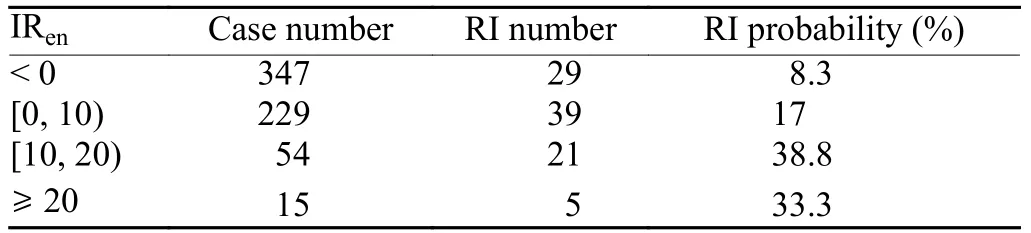
Table 4. The probability of TC RI in different IRen intervals based on the independent samples from 2019 to 2020

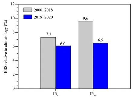
Fig. 7. The skill of two TC RI probability models (IRe and IRen) relative to climatology for dependent samples from 2000 to 2018 (gray bar)and independent samples from 2019 to 2020 (blue bar). The difference between IRen and IRe model is that the TC intensity is taken into account or not.

Table 3. The probability of TC RI in different IRen intervals from 2000 to 2018

Figure 9 evaluates the forecasting skill of the model IRencomprehensively by calculating the probability of detection (POD), probability of false detection (POFD),and Peirce skill score (PSS). The POD is the fraction of the observed number of RI cases that were forecast correctly. The POFD is the ratio of the number of cases that an RI was forecast to occur but did not, divided by the total number of cases that RI did not occur. The PSS was applied in previous studies to show the performance of the linear weighting RI index, which is defined as the difference between the POD and POFD (Kaplan et al.,2010; Shu et al., 2012). In brief, the POD, POFD, and PSS of a perfect model should be 1, 0, and 1 respectively. In this study, the value of IRengreater than 20 is considered as a threshold for TC RI for cases from 2000 to 2018 and TC Chanthu, and 10 for cases from 2019 to 2020 as the 2-yr sample size is small. The POD of three groups is greater than 20%, and up to 66.7% for TC Chanthu. The POFD of IRenis performed quite well,which is less than 8%. Shu et al. (2012) developed a linear weighting RI index (RII) for the WNP TC, and the averaged PSS of the RII is about 0.1. The PSS of IRenis greater than 0.15 for these three groups of cases and up to 0.64 for TC Chanthu, indicating that IRenhas skill for the WNP TC.

5. Summary and discussion

In this study, the effect of TC environmental conditions on the TC intensification rate is investigated. The WNP TC best track data from JTWC and surrounding environmental fields from the NCEP final analysis data over 2000-2018 are employed. Two TC RI probability models are developed by utilizing least squares analysis.

The RI is defined as the maximum surface wind speed increase of 30 knots over 24-h period. There are 6307 TC cases in the WNP from 2000 to 2018, of which 856 cases occur with RI, accounting for 13.6%. In order to figure out the relative role of different surrounding environmental variables on the TC IR, the BDI method is applied in this study to rank environmental variables that are statistically significant at the 95% confidence level.Following six variables are selected as the TC RI predictors:TS-T0, OHC, VUS, Lon - Lat, ω400, and RH500.Specifically, a TC with high environmental SST, OHC,and low upper-level temperature, is more likely to occur RI. Moderate easterly shear is more favor for the TC intensification than westerly shear. Intensifying cases are located mostly equatorward of 20°N while weakening cases are mainly located in the northwest of intensifying cases. Relative humidity and vertical velocity at middle level are good indicators that can separate the intensification cases from the non-intensification cases.

Based on these six predictors, the least squares method is adopted to develop a probability prediction model for the TC RI by using cases from 2000 to 2018. The correlation coefficient between the probability model IReand the observed IR reaches 0.523. After considering the effect of TC intensity on the TC RI, an intensity-dependent model IRenis developed and shows better performance. When IRenis greater than 20, the probability of TC RI at that moment reaches 40.9%. Both IReand IRenare skillful relative to climatology for the WNP basin, and the skill of IRenis higher. Moreover, independent verification for IRenis conducted based on samples derived from 2019 to 2020 and TC Chanthu (2021). IRencan capture the characteristic of the surrounding environment well and is a good indicator of IR.

In the current study, we concentrate on the effect of the surrounding environment on the TC RI. It should be pointed out that the occurrence of TC RI is not only related to the environmental field, but also related to the structure of TC itself. As the horizontal resolution of the reanalysis data is not high enough, it is difficult to use the reanalysis data to study the impact of the TC internal structure on RI. Although the probability model IRenshows some forecasting skills, due to the lack of description of the internal structure of TCs, there may be an upper limit on the predictability of the TC intensity change rate. This problem prompts us to build a TC database by using high-resolution numerical model and explore the relationship between the internal structure of TC and IR in the future study.

Acknowledgments.We thank the editor and anonymous reviewers for their constructive comments and suggestions. We acknowledge the High Performance Computing Center of Nanjing University of Information Science & Technology for their support to this study.