Zhenkun Liao,Yuliang Zhao and Sheng Dong

Abstract Nonlinear time-domain simulations are often used to predict the structural response at the design stage to ensure the acceptable operation and/or survival of floating structures under extreme conditions. An environmental contour (EC) is commonly employed to identify critical sea states that serve as the input for numerical simulations to assess the safety and performance of marine structures.In many studies,marginal and conditional distributions are defined to construct bivariate joint probability distributions for variables, such as significant wave height and zero-crossing period. Then, ECs can be constructed using the inverse first-order reliability method(IFORM).This study adopts alternative models to describe the generalized dependence structure between environmental variables using copulas and discusses the Nataf transformation as a special case.ECs are constructed using measured wave data from moored buoys.Derived design loads are applied on a semisubmersible platform to assess possible differences. In addition, a linear interpolation scheme is utilized to establish a parametric model using short-term extreme tension distribution parameters and wave data, and the long-term tension response is estimated using Monte Carlo simulation.A 3D IFORM-based approach,in which the short-term extreme response that is ignored in the EC approach is used as the third variable,is proposed to help establish accurate design loads with increased accuracy.Results offer a clear illustration of the extreme responses of floating structures based on different models.

Keywords Design loads;Mooring system;IFORM-based approach;Copulas;Nataf transformation;Short/long-term extreme response

1 Introduction

Marine resource development, including the extraction of petroleum resources and the harnessing of wave energy and offshore wind energy,is an area of active research focus in ocean engineering.Floating structures and mooring systems must be designed to withstand the complex marine environmental loads that result from wind, waves, currents,and ice to support activities related to marine resource development. Nonlinear time-domain simulations are often performed to predict extreme response levels at the design stage to ensure the acceptable operation and survival of these floating structures in extreme conditions.Design levels must be defined on the basis of reasonable extreme metocean design criteria to perform an accurate assessment of the floating structures. By studying the joint distribution/statistics of underlying environmental parameters,our goal is to establish accurate design loads for floating structures with a mooring system design assigned with a prescribed target return period.

In general,the safety of the floating structure under consideration must be assured over the period of the planned operation.Based on the statistical analysis for environmental variables, the wind or wave parameters associated with a 50-or 100-year return period are often adopted as the design basis for extreme conditions for floating structures(DNV 2012). The dependency between various ocean parameters should be considered to assess structural responses accurately and to obtain a realistic estimation of reliability. For this purpose, bivariate or multivariate joint probability models are commonly constructed. Although different joint distribution models have been proposed in practice, no unifying benchmark standard for establishing joint distribution models for metocean parameters exists (Jonathan and Ewans 2013).A hybrid log-normal-Weibull conditional distribution for significant wave height and wave period proposed by Haver (1985) is widely employed for North Sea sites. Further investigations on joint distributions for other metocean parameters based on conditional models have been the subject of studies by other scholars(Belberova and Myrhaug 1996; Bitner-Gregersen 2005;2015). Dong et al. (2013) proposed a bivariate maximum entropy distribution for significant wave height and the associated spectral peak period. On the basis of copulas and maximum entropy margins,Dong et al.(2017)constructed multivariate maximum entropy distributions for wind speed, current velocity, and significant wave height for wind turbines. Tao et al. (2013) estimated the design parameters of wave height and wind speed using bivariate copulas. Manuel et al. (2018) showed how the same data can be used to establish different distribution models for significant wave height and spectral peak period and, in turn,how different environmental contours(ECs)could be constructed using parametric and nonparametric approaches. Moreover, they compared contours for Nataf, Rosenblatt, and different copula family dependence structures.Vanem(2016b)presented joint statistical models for significant wave height and wave period based on copula techniques. Their results illustrated the role of modeling choice in introducing uncertainty.

The adopted EC method is based on the inverse first-order reliability method (IFORM) and can be employed to establish design loads associated with a specified return period. Other algorithms for EC construction exist (Ross et al.2020;Chai and Leira 2018).They include the inverse second-order reliability,direct sampling contour,and highest density contour methods. The main advantage of EC method is the decoupling of the structural response from the environment.As a result, the target reliability index and return period are related only to the environmental variables.This result effectively reduces nonlinear time-domain response simulations. Haver and Winterstein (2009) demonstrated the construction of EC lines for significant wave height and peak period using conditional models. Silva-González et al. (2013) developed 3D ECs for the significant wave height,peak period,and wind speed using a Nataf transformation approach. Huseby et al. (2013) presented an approach for the construction of ECs for significant wave height and peak period based on direct Monte Carlo simulations. Monte-Iturrizaga and Heredia-Zavoni (2015)applied copulas to develop ECs for bivariate metocean variables. Once ECs are constructed, the design loads correspond to the maximum structural response from all candidate choices of parameters along contour lines.

The methods described above do not explicitly consider the uncertainty in the structural response if the design loads are obtained through the 2D EC approach.Therefore,a 3D IFORM-based approach that explicitly includes the structural extreme response as a random variable is also considered in this study.First,the ECs for a selected site are constructed using measured wave data from moored buoys on the basis of various models, and EC-based design loads are derived. Then, the long-term extreme response of a floating structure is established through Monte Carlo simulation combined with the constructed parametric model for short-term extreme response distribution parameters and wave data. The results obtained from the approaches based on 2D EC, 3D IFORM, and long-term extreme responses are compared.

2 IFORM-based EC approach

Winterstein et al. (1993) proposed an EC approach to derive the environmental parameters for extreme structural response analysis based on IFORM. In this case, assume a vector of two random environmental variablesX= (Hs,Te)corresponding to a target return periodTror a probability of response exceedancePfto which one can associate a reliability indexβas follows:

whereTsrepresents the interval of the sampling data in the 2D EC method or the duration of the response simulation in the 3D method in h.A 3 h dynamic response simulation is usually performed to ensure the stability of statistical characteristics for floating structures.Moreover,Tr,the target return period, is defined as a part of the design criteria in years.In reliability-based design,one is interested in estimating the value of structural response capacityyc, which will ensure thatPf=P(y>yc).The reliability indexβrepresents the shortest distance from the origin in a standard normal space to the failure domain.The variables transformed from the original random variables follow a standard normal distribution in the standard normal space.

In the IFORM approach, the reliability indexβdenotes the constant distance(or radius)in a standard normal space.Then, the EC line can be expressed in this normal space with a constant radiusβ, where the bivariate independent random variablesz= (z1,z2) on the contour vary with the angleθas follows:

Moreover,the original variablesx=(x1,x2)in the physical space can be transformed from the vector of random variableszin the standard normal space using the Rosenblatt transformation:

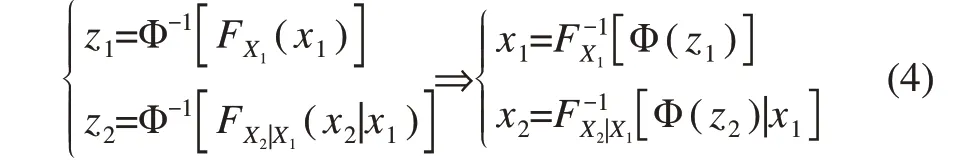
where Φ(·) denotes the cumulative distribution function(CDF) of the standard normal distribution,FX1(x1) andFX2|X1(x2|x1) represent the CDF of the original variablex1and the conditional distribution ofx2givenX1=x1,respectively. Figure 1 provides an illustration of the ECs for two return periods in the standard normal space (z) and in the corresponding physical space (x). For a 2D case, EC is a contour “line” rather than a “hypersphere,” which is used later for high-dimensional cases.

2.1 Conditional joint environmental model

For the construction of an EC, wave-related variables should be described using a joint distribution model.A conditional joint distribution model of significant wave height and peak period is employed as(Vanem and Bitner-Gregersen,2012)

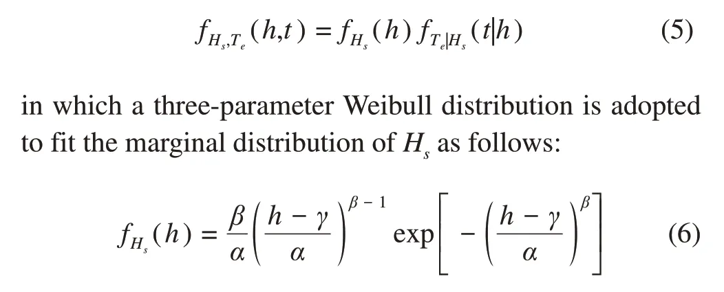
and a conditional log-normal distribution is chosen to representTegivenHs. The conditional distribution parameters depend on the value ofHs:

Thus, the joint description for the wave-related random variablesHsandTecan be constructed by fitting parametersα,β,γ,ai,bi, andcifori= 1, 2 to the available data.Note that the marginal distribution ofHsand the conditional distribution ofTeshould be determined using the goodness-of-fit test.The test shows that the Weibull and conditional log-normal distribution accurately describe the sample data at a given level of significance in this study.

2.2 Copula theory

A multivariate joint distribution can be established by combining univariate marginal distributions for each random variable with copula functions that describe the dependence structure between these variables. Copula models are commonly used for joint distributions construction due to their great flexibility, in which the marginal distribution of environmental variables can be arbitrary.Moreover,the correlation or dependence structure of environmental variables can be considered separately using copula functions.Assume thatFXi(xi) is the marginal distribution forxi,which is one variable from the vector ofnrandom variablesx=(x1,x2, …,xn) . The joint distribution functionHX1,···,Xn(x1,x2,…,xn)ofxcan be expressed in accordance with Sklar’s theorem(Sklar 1959)as follows:

Figure 1 ECs in the standard normal space(z)and in the physical space(x)for 50-and 100-year return periods

whereC(·)denotes a monotonic and nondecreasing copula function that can be written in terms of the joint distribution and the inverse marginal CDF of each variablexi:

A parameter,namely,θ,that is used to describe a selected copula function helps describe the correlation or dependence structure between random variablesxfor a selected copula functionC(·). The maximum likelihood method is commonly employed to estimate unknown parameters.For bivariate situations,θcan be obtained on the basis of Kendall’sτwhich is used to represent the degree of dependence of variables:

whereais the number of concordant pairs,brepresents the number of discordant pairs,ndenotes the total number of data pairs.

2.3 Contour plots using copula

The radiusβof the hypersphere in the standard space can be determined using Eq. (1) and Eq. (2) based on the given target return periodTr.Then, ECs can be constructed by transforming the original environmental dataxfrom the standard normal spacezusing the Rosenblatt transformation. By combining Eq. (13) and Eq. (4), the CDFs ofxcan be obtained by the inverse transformation of the copula functionsC-1(·)as follows:

For the bivariate case, solving the partial derivatives of the copula function is the most important step,C(v|u) =∂C(u, v)/∂u.A wide range of copula functions can be adopted to establish the bivariate joint distribution of the wave-related datasets. These functions include Archimedean and elliptic copula functions. Montes-Iturrizaga and Heredia-Zavoni (2015) provided a detailed description of the method for constructing ECs using copulas. In the present study,four kinds of copula functions(Frank,Clayton,Ali-Mikhail-Haq [A-M-H], and independent copula models)(Nelsen 2006;Venter 2002) are considered and applied for EC construction. The adopted copula models and corresponding variablevin physical space are listed in Table 1.

2.4 Nataf transformation

Generally, the original statistical wave data can provide basic information about marginal distributions and the correlation structure of environmental variables. The Nataf distribution model is a common technique for constructing joint descriptions for original data consistent with the prescribed marginal distributions and correlation structures(Silva-González et al. 2013). The Nataf transformation method is equivalent to a Gaussian copula, where the random variables are noted to be mapped onto correlated standard normal variables, provided that their joint density is defined by a Gaussian copula. The Nataf model offers a transformation from the original variable space into an independent standard normal space:

wherexis the vector of target variables,x=(x1,x2,‧‧‧,xn)T;Fi(xi) represents the CDF of each environmental randomvariablexi;yis the standard normal random variable vector that corresponds toxandy= (y1,y2, ‧‧‧,yn)T; and Φ(·)and Φ-1(·)are the CDF and inverse CDF of a standard normal random variable,respectively.

Table 1 Adopted copula models and variable expression in physical space

Silva-Gonzláez et al. (2013) presented an EC approach using the Nataf transformation model. In this case, the expression forvis given as

whereρis the Pearson's correlation coefficient of the variables in the transformed standard normal space.

2.5 3D IFORM-based approach

The design load of a mooring system for a specified return period is evaluated in this study.Note thatFR|Hs,Te(r|h,t),which denotes the conditional CDF of the extreme tension variable givenHsandTe,must be established using response simulations. Design loads can be derived using integration combined with Monte Carlo simulation, as will be discussed.

In the 2D EC method,design loads corresponding to critical sea states can be obtained by carrying out numerical simulations for the sea states corresponding to the (Hs,Te)values lying on the 2D EC and selecting the largest median response value. Although the 2D method is approximate because it does not consider response variability,it is computationally very efficient.

The 3D approach couples the description of the environmental variables with the extreme response of the floating structure (Saranyasoontorn and Manuel 2004). However,compared with other approaches,it takes significantly more time to explore the extreme response of the system, even though its final results are more accurate.The 3D IFORMbased model, in which the short-term extreme response is regarded as the third random variable, can be expressed as follows:

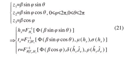
whereδandρare the short-term extreme tension distribution parameters that are sensitive to wave conditions. In the conventional 2D EC approach,z3= 0 andΦ(z3) =Φ(βcosφ) = 0.5. Thus, the extreme tensionris adopted as the median value from this equation, and (ĥs,t̂e) is adopted as the critical sea state along the 2D EC that leads to the largest median extreme tension response.Various joint models can be employed to construct 2D ECs.In the 3D IFORMbased approach, short-term extreme response uncertainties are considered,and the design loads are adopted as the largest response (the point corresponding to the largest third variable on the hypersphere).A constructed parametric model for extreme distribution parameters and any wave data makes this idea feasible and improves computational efficiency.

3 Long-term extreme response analysis

3.1 All-sea-state approach

The most precise approach for predicting the extreme response is the full long-term analysis. All conceivable sea conditions and the corresponding nonlinear time-domain numerical simulations of mooring system should be considered to estimate the design tension, wherein each sea state and response is regarded as a stochastic process.Assessing the long-term extreme response of mooring systems under wave excitation loads requires the long-term probability distribution of environmental variables and the short-term extreme response probability distributions for different environmental conditions. The long-term distribution of mooring line tension can be obtained using the following integral:

where(hi,ti)is the discrete sample of the random wave data that follow a specified joint distribution obtained using random number generation techniques. Moreover,nis the total number of generated random variables.

In this study, the inverse CDF method is adopted as the random number generation technique. This approach involves two steps: (a) for each sea state,nrandom samples(s1,s2), which are uniformly distributed between 0 and 1,are generated using Monte Carlo simulation; (b) then, the random wave data can be produced using the inverse transformation method:

The basic principle is that the CDF for random samples(x1,x2) corresponds to the random samples (s1,s2), as depicted in Figure 2.

3.2 Short-term peak response

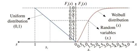
Figure 2 Illustration of the inverse transformation method for the generation of random environmental variables

The determination of functions for the short-term extreme tension of mooring systems is described in this section.The time history response during wave loading has numerous peak samples.Taking the significant ones from these peak values is important to form a short-term extreme distribution. Several approaches have been introduced to define the distribution of the extreme response (Stanisic et al.2018;Xu et al.2019).These approaches include the global maxima method and the peak-over-threshold (POT) method. The extreme level obtained from the global maxima method is usually adopted as a benchmark, in which the maxima are adopted as extreme values from a series of time histories with various seeds. This method is time-consuming because numerous numerical simulations should be conducted for a single-wave condition with different seeds. In contrast to the global maxima method,the POT method can provide an approximate result using a single time-domain response under a single-wave condition.In this method,all peak tension values exceeding a prescribed thresholdu0are gathered to determine a distribution model. In this case,only the largest 50%of the extremes obtained for each sea state are considered because we are interested in the tail of the distribution (Liu et al. 2019). Figure 3 shows extreme response sampling using the POT method.

Figure 3 Extreme value sampling using the POT method

Once the short-term extreme response distribution of the mooring system is determined, a discrete grid map comprising a mesh of a specific number of points (Hs×Te) is used for the investigation of the relationship between distribution parameters and wave variables.Then,the parameters of the extreme response for any given environmental conditions can be predicted using the linear interpolation scheme. The long-term extreme response CDF can be calculated on the basis of the Monte Carlo simulation and the established parametric model.

4 Case study

The purpose of this study is to evaluate the extreme response of mooring lines for a floating structure and to establish design loads for a specified return period.This case describes the techniques for determining design loads for the mooring systems of floating structures on the basis of the conventional 2D EC approach, 3D IFORM-based approach,and long-term extreme response model.The 2D ECs are constructed using various joint distribution models.The aforementioned conventional joint distribution models combined with IFORM are applied to describe the wave variablesHsandTethat are related to different target return periods.Monte Carlo simulation combined with a parametric model for extreme distribution parameters and wave data is employed to calculate the long-term extreme response of a semisubmersible platform mooring system. The section shows the variability in the prediction of design loads using various models even with the same data.

4.1 Wave data and structural description

Figure 4 Scatter plot showing the data on the metocean variables Hsand Te at National Data Buoy Center Station 46022

Figure 5 Density function fitting for Hs

Significant wave height (Hs) and energy period (Te) data are collected from the National Data Buoy Center Station 46022.This location is an offshore site with a 675 m water depth in Northern California.A total of 122 467 hourly observations from January 1, 1996, to December 31, 2012 are provided from this bouy (Eckert-Gallup et al. 2016). The scatter plot of the wave data is shown in Figure 4.A threeparameter Weibull distribution model is adopted to fit the significant wave height. The fitting result is depicted in Figure 5, which shows that the density curve fits the observations well.The fitting results of the conditional probability density ofTegiven differentHsare shown in Figure 6.The conditions forHs=0.5-1.0,2.5-3.0,4.5-5.0,and 6.5-7.0 m are depicted in this figure.The estimated parameters of the conditional joint model using the maximum likelihood method for the selected site are presented in Table 2 and Table 3. The fitting curves of log-normal distribution parameters for given classes ofHsare shown in Figure 7.The least squares method is adopted to determine the relationship between distribution parameters and wave height.Although there exist other methods for parameter estimation (Vanem et al. 2019; Haselsteiner et al. 2019; Vanem and Huseby 2020) that have significant effects on EC results, the purpose of this study is to show the comparison of design loads obtained through approaches based on 3D IFORM, long-term extreme response, and conventional 2D EC.Therefore,the differences caused by different parameter-estimating algorithms are not discussed in this study.

To illustrate the application of various models to estimate design tension, a semisubmersible platform composed of two pontoons, four columns, four braces, and 12 mooring lines and designed for service at a depth of 500 m is introduced in this section.Table 4 lists the primary geometric details of the moored platform.Table 5 presents the main properties of the mooring lines. A one-quarter finite element model is established with the hydrodynamic analysis software ANSYS/AQWA and is depicted in Figure 8. The 3D radiation/diffraction theories and the Morison equation are employed to quantify the wave loads and structural dynamic responses of large-scale coupled floating system.The compatibility of the body motions and mooring tensions at the fairleads is considered to solve the dynamic behavior of the coupled floating system for each integration step.The body motions at the fairlead are solved first and then are used to calculate the top tensions of mooring lines(which can also be transferred to the floating body as external forces).The simulation length for all cases in this study is 10 800 s(3 h)with a time interval of 0.2 s.The extreme design tension of the mooring lines excited by wave loads originating from one direction is estimated herein.

4.2 Long-term extreme tension response

Figure 6 Conditional probability density functions fitting for Te given Hs

Table 2 Weibull distribution parameters for the joint environmental model(Hs)

Table 3 Conditional log-normal parameters for the joint environmental model(Te)

The dynamic responses of the coupled floating structures and mooring systems under irregular wave conditions are simulated using the ANSYS/AQWA software.The random sea conditions depicted in Figure 4 are simulated as a stationary random process, and the extreme tension distribution of the mooring lines can be obtained from time-domain simulations combined with statistical analysis. The shortterm extreme response is predicted using the POT method(Agarwal and Manuel 2009).A total ofNs= 9 × 17 (Hs×Te)=153 simulations are performed to conduct the interpolation scheme. In these simulations, the wave heights range from 1 m to 9 m and the wave periods range from 4 s to 20 s(solid blue dots in Figure 4). Mooring tension peaks can be defined from a single time series by utilizing the POT method, in which only the individual top peaks above a given threshold are selected and fitted. Several algorithms, such as the mean residual life plot and root square error methods,have been proposed for optimal threshold selection.A general threshold at the mean plus 1.4 standard deviation level or at the 50%-95%percentile of the total top peaks is also commonly adopted. Stanisic et al. (2018) investigated the sensitivity of the peak distribution method in the selection of different portions of the peaks(top 10%,20%,30%,40%,and 50%). In the present study, the upper 50% of the individual peak response of a single time series is selected, and various extreme distribution models are employed to fit the top peaks. Generally, the GPD is the preferred model for POT.However,the three-parameter Weibull distribution has been pointed out to be possibly a better choice than the GPD.Moreover,the Gumbel model is extensively used for the extreme tension fitting of mooring lines. The Gumbel distribution is chosen to describe the short-term extreme response as follows(Baarholm et al.2010):

Figure 7 Fitting curves for distribution parameters given Hs

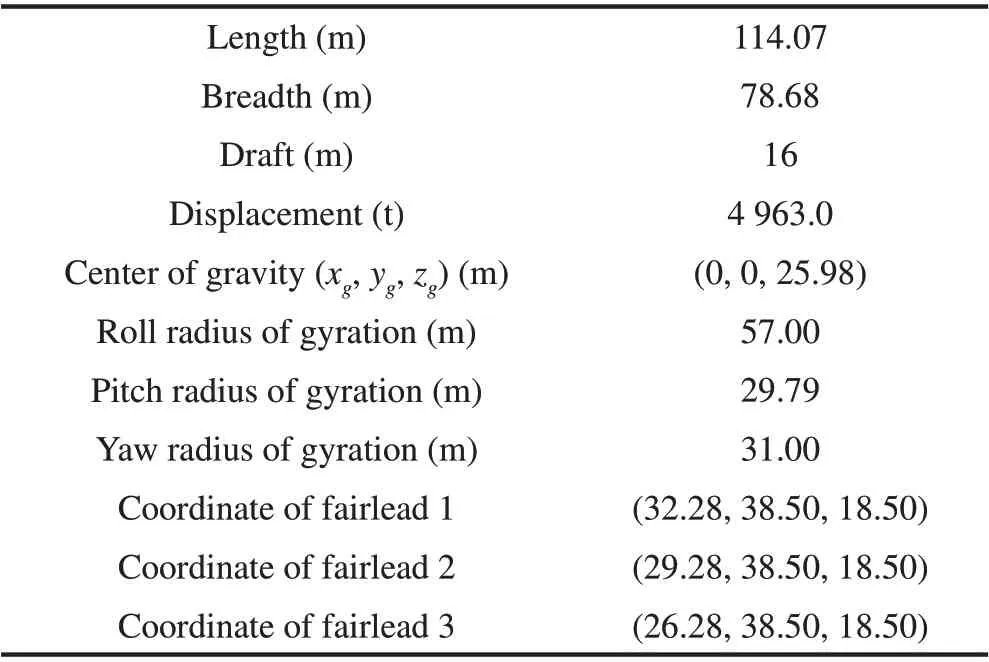
Table 4 Main characteristics of the semisubmersible platform

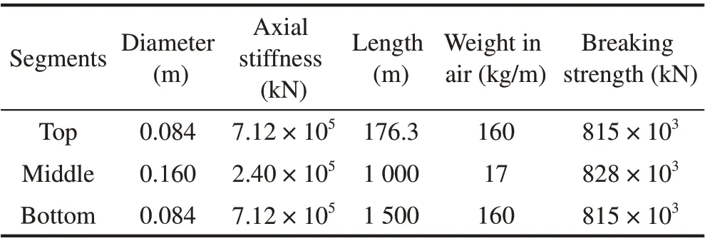
Table 5 Main parameters of the catenary mooring line

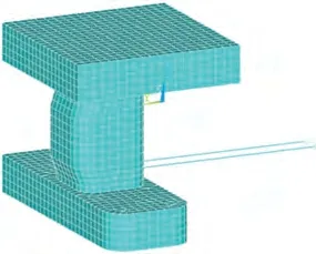
Figure 8 Semisubmersible hydrodynamic model (the one-quarter model is shown due to symmetry)

where (δ,ρ) denote the location and scale parameters, respectively.The fitting for the POT-based extreme values is depicted using diagnostic tests.The short-term extreme distribution test diagrams, including exceedance probability and density plot, for one given environmental condition withHs= 7 m,Te= 13 s are depicted in Figure 9.As shown in the diagrams,the extreme values,which are represented using blue scatter points and histograms, fit the corresponding empirical curves well.The density histogram indicates that the density curve matches the original data well.Eq.(25)is based on the assumption that the peaks above the chosen threshold are independent. If a load nonexceedance probability leveldis of interest, the corresponding load fractilerdbased on the POT distribution associated with a nonexceedance probabilityd1/n0can be estimated as (Agarwal and Manuel 2009):

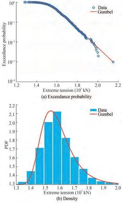
Figure 9 Diagnostic plot of the Gumbel distribution of short-term extreme tension under a sea state with Hs=7 m,Te=13 s

The discrete grid map shown in Figure 4 comprising a mesh ofNs=153 points(Hs×Te)is used for the investigation of the relationship between (δ,ρ) and wave parameters (Hs,Te). These points cover all possible wave conditions produced using a random data generation technique to avoid performing a large number of nonlinear time-domain dynamic response analyses for each random sea condition.First,153 3 h nonlinear time-domain dynamic analyses of the floating structure system were performed and short-term extreme distributions of POT-based response were fitted. The relation between (δ,ρ) and (Hs,Te) is obtained and depicted in Figure 10. The results indicate that for a givenHs, the distribution parameters have a similar trend asTe, and no suitable simple explicit expressions, can describe the relation accurately; hence, the parameters of the short-term extreme tension distribution for any other wave condition were calculated using a linear interpolation procedure which is implemented using MATLAB. The total number of discrete random variables for long-term integral calculation in Eq.(23)is taken as 1×105.The random environmental variables are generated using the inverse CDF method combined with the parametric model.The CDF of the long-term extreme tension of the most loaded mooring line is obtained and shown in Figure 11.The random wave data generated using the inverse CDF method is presented in Figure 12. The number of higher wave heights is lower than the original data.This result indicates that the tail fitting forHsis imperfect.However,we still think that the results of the long-term analysis are reliable due to the low occurrence probability for the high wave height region.The discrete number is sufficient,as depicted in Figure 11.A large discrete number will not improve accuracy with the increase in computation time.

Figure 10 Fitting curves for the distribution parameters associated with wave data

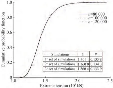
Figure 11 Long-term extreme cumulative distribution for the most loaded mooring line

Figure 12 Random wave data generated using the inverse CDF method

4.3 Estimation of design loads

4.3.1 2D Environmental contour lines

Different approaches for EC construction are considered.The conditional model uses a Rosenblatt transformation based on the marginal and conditional distributions forHsandTe,whereas the Nataf model is based on the use of the marginal distributions forHsandTealong with Pearson’s correlation coefficient.Kendall’sτis estimated using Eq.(14)to account for the dependence structure betweenHsandTewith the copula models (Frank, Clayton, A-M-H, and independent). The high value ofτ= 0.29 indicates that the dataset has a relatively strong degree of dependency.Figure 13 shows the EC plots of (Hs,Te) for a 20-year return period considering the different models. The ECs do not fit the original wave data perfectly.The standard copula has only one degree of freedom and could not capture theHs/Tedependence correctly.The extraparametrized copulas are employed for ECs in a previous study (Vanem,2016a). This study does not focus on the conventional 2D EC approach but instead provides a highly detailed comparison of the approaches based on 3D IFORM, long-term extreme responses, and 2D EC. In the 2D EC method, the critical design sea state can be obtained by considering the point along the contour that corresponds to the largest median response. The critical design environmental conditions and 2D EC-based extreme response values are presented in Table 6.

Figure 13 ECs for(Hs,Te)using various models

4.3.2 Design load estimation using the 3D IFORM-based method

The 3D IFORM-based model includes the short-term extreme tension and environmental variables for estimating design loads. The constructed 3D sphere is depicted in Figure 14. Similar to that in the 2D EC approach, the entire sphere should be searched in this model to find the largest extreme tension as the design level.Given that the shortterm extreme tension response is sensitive to wave height and wave period, as depicted in Figure 10, the constructed parametric model for response distribution parameters and waves is important for 3D model establishment.As shown in Figure 14,in consideration of their dependency,the wave data and mooring line tension are transformed from the standard normal space for the 20- and 100-year return periods.The design levels obtained using the 3D IFORM-based approach are 2 603.1 and 2 864.8 kN,respectively.Table 7 lists the detailed results for design loads and critical sea states.

Figure 14 3D IFORM-based model and design loads for the 20-and 100-year levels

4.3.3 Design load estimation using the long-term response method

The design loadsrqcorresponding to different return periods(target percentiles)can be defined as follows(Stanisic et al.2018):

Table 6 Design load estimates based on the 2D EC method

Table 7 3D IFORM-based model results for different return periods

wheretandTare the response sample time length and target return period,respectively.

The POT-based load extremes during the 3 h dynamic response in time-domain simulations are adopted as the target extreme value. Thus, herein, we obtaint= 3 h andT= 20, 50, and 100 years.The extreme design values predicted using Eq.(28)are depicted in Figure 15.In this case,for a 100-year return period, the percentile is calculated to beξ= 1-3/(100 × 365 × 24), and the long-term design load is found to be 3050.1 kN. Compared with the EC approach,in which the mooring line tension is analyzed using only the design critical environmental condition as input and the short-term median extreme tension is adopted as the desired output, this procedure provides a more accurate assessment of design loads for floating structures because the long-term extreme-based model accounts for the sequence of all possible sea states and couples the structural response with environmental variables.The expected longterm design values for three return periods are presented in Table 8.

Figure 15 Estimation of design loads based on the long-term extreme response

Table 8 Long-term response-based model results for different return periods

Tables 6-8 summarized different design loads obtained using various abovementioned models.The results show that the load valuesrqincrease with the target return periods as expected, whereas the design points for wave data do not follow this trend because the variableTe, is not positively correlated with the dynamic response of floating structures as shown in Figure 10. The design loads estimated using 2D EC-based models,including the conditional joint distribution model, Nataf transformation, and copula models,show different extreme levels. For the 20-year return period,the maximum difference in extreme tension is approximately 3.77% because the largest short-term median extreme values are regarded as design loads along ECs, and the ECs are discrepant due to the different joint probability models for the same wave data. Meanwhile, great differences are noted using 3D IFORM-and long-term extremebased models when the models consider the short-term extreme response and environmental condition uncertainties.The 20-year extreme tension obtained with the long-term response model is approximately 37.20% higher than that acquired with the 2D design level (conditional joint model) and just approximately 8.15% higher than that found with the 3D-IFORM-based design level.These results indicate that the influence of long-term environmental loads on floating structures should be included in design level estimation, especially in cases with large response variability.Similarly,the variability in the short-term extreme response,which leads to conservative design loads for floating structures, should be considered in IFORM-based approaches.Figure 16 illustrates the design load levels obtained using the various presented models. It shows that the discrepancy between the loads derived from the models that consider the response uncertainties and those from the ECs is non-negligible.Thus,for floating structures with complex hydrodynamic responses,design load estimation based on the longterm response model, in which all possible sea states during long service life are considered,must be performed due to the observation that usually,no significant positive correlation exists between variables,including wave data and extreme structural response.

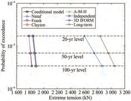
Figure 16 Extreme tension for the 20-, 50-, and 100-year return periods based on various models

5 Conclusions

The dynamic response analysis of a semisubmersible platform was conducted to estimate design loads. A conventional 2D EC approach based on various dependence models,including the conditional Rosenblatt model;Nataf transformation; and the Frank, Clayton,A-M-H, and independent copulas, was adopted to identify the critical sea state and establish the 20-,50-,and 100-year design loads.The extremes of the tension of the mooring system were analyzed using the POT method,and a Gumbel distribution was found to fit the POT-based extremes well.A limited set of 153 sea states was discrete,and the stochastic parameters of the shortterm extreme response were investigated as a function ofHsandTe, in which a linear interpolation scheme was utilized to construct the parametric model.The long-term extreme response was obtained through a discrete approach in combination with the Monte Carlo method and parametric model.A 3D IFORM-based model was also constructed by considering the short-term extreme response as the third variable.The results obtained by means of 2D EC,the 3D IFORM-based approach,and the long-term extreme response method revealed that the selection of different models had a significant effect on the resulting critical sea conditions and the corresponding design values.The full longterm analysis that considers all conceivable sea states can provide the most accurate assessment.The EC method that uncoupled the structural response and environmental variables was efficient and provided design load results that can be inaccurate and unconservative compared with the results provided by the 3D IFORM-based and long-term load models.The inclusion of uncertainties in the short-term extreme tension load conditional on environmental variables yielded considerably higher return levels than the conventional EC approach and is recommended for practical applications.

FundingSupported by the National Natural Science Foundation of China under Grant No.52171284.

Open AccessThis article is licensed under a Creative Commons Attribution 4.0 International License, which permits use, sharing,adaptation, distribution and reproduction in any medium or format, as long as you give appropriate credit to the original author(s) and thesource, provide a link to the Creative Commons licence, and indicateif changes were made. The images or other third party material in thisarticle are included in the article's Creative Commons licence, unlessindicated otherwise in a credit line to the material. If material is notincluded in the article's Creative Commons licence and your intendeduse is not permitted by statutory regulation or exceeds the permitteduse, you will need to obtain permission directly from the copyrightholder. To view a copy of this licence, visit http:/creativecommons.org/licenses/by/4.0/.