Utku Cem Karabulut,Yavuz Hakan Özdemir and Barış Barlas

Abstract Recently, computational fluid dynamics (CFD) approaches have been effectively used by researchers to calculate the resistance characteristics of ships that have rough outer surfaces. These approaches are mainly based on modifying wall functions using experimentally pre-determined roughness functions.Although several recent studies have shown that CFD can be an effective tool to calculate resistance components of ships for different roughness conditions, most of these studies were performed using the same ship geometry (KRISO Container Ship). Thus, the effect of ship geometry on the resistance characteristics of rough hull surfaces is worth investigating.In this study,viscous resistance components of four different ships are calculated for different roughness conditions.First,flat plate simulations are performed using a previous experimental study for comparison purposes. Then, the viscous resistance components of three-dimensional hulls are calculated.All simulations are performed using two different turbulence models to investigate the effect of the turbulence model on the results. An examination of the distributions of the local skin friction coefficients of the DTMB 5415 and Series 60 showed that the plumpness of the bow form has a significant effect on the increase in frictional resistance with increasing roughness.Another significant finding of the study is that viscous pressure resistance is directly affected by the surface roughness.For all geometries,viscous pressure resistances showed a significant increase for highly rough surfaces.

Keywords surface roughness;frictional resistance;ship resistance;computational fluid dynamics;RANS

1 Introduction

Maritime transport is of great importance in global trade. More than 80% of commercial products in volume and more than 70% in financial terms are carried by ships(UNCTAD 2017). However, ships, which are the world’s largest means of transportation, use fossil fuels as energy sources. The International Maritime Organization (IMO)imposes strict regulations to reduce greenhouse gas emissions related to fossil fuel consumption on ships,with measures and regulations being put in place with the aim of reducing greenhouse gas emissions by 20% by 2020, 25%by 2025,and 30%by 2030.Increasing the energy efficiency of ships is the primary priority of the IMO and the energy efficiency design index, which came into force in 2013 and is defined as the most important technical regulation for newly built ships (IMO 2009; Longva et al. 2010). In addition, the economic recession in the maritime industry in recent years has forced companies to reduce their operational costs. One way to overcome this problem is to reduce the cost of fuel by lowering total resistance with a well-designed hull.

A ship is subjected to a resistance force against the direction of movement. Resistance consists of two main components: frictional resistance and residuary resistance(Molland et al. 2011). Frictional resistance, as the name implies, occurs due to tangential fluid forces and usually accounts for most of the total resistance. Friction resistance makes up about 80% of the total resistance in lowspeed ships such as oil tankers and around 50% in highspeed ships such as container ships (Lackenby 1962). Predicting ship resistance with high precision is critical for the design phase and the operation of the ship.Correct estimation of frictional and residual resistance forces acting on the ship enables the design of ships with low fuel costs and high energy efficiency. Thus, environmental pollution caused by transportation activities at sea can be reduced.

The frictional resistance of a ship depends on the geometry of the hull and the roughness of its outer surface.As surface roughness increases, resistance increases. The outer surfaces of the ships are constantly exposed to biofouling,which causes a constant increase in surface roughness.Biofouling is considered an important problem in shipping and is defined as the colonization of the outer surface of ships by marine species such as mussels.Antifouling coatings have been developed to deal with this problem.

The roughness-resistance relationship has attracted the attention of many researchers since the second half of the 18th century. The first studies investigating the effect of surface roughness on frictional resistance were conducted by Froude (1872, 1874). The first comprehensive experiment to investigate the effect of contamination on resistance was conducted by McEntee(1915).Within the scope of the experiments,flat plates were painted with anticorrosive paint and kept at sea for a while. Experiment results showed that the frictional resistance increased four times in the plates exposed to sea water for 12 months.

Another early study that provided detailed information about the increase in ship resistance due to roughness was conducted by Lackenby (1962), presenting the resistance properties of an 18 000 DWT tanker ship operating at 14 kn service speed and a channel ship operating at 22 kn service speed. Findings show that the increase in the resistance force due to biological contamination from a three-year operation on the tanker ship is 31%,and the increase in resistance force on the channel ship from a four-year operation is 21%.The study also found that regular maintenance and repair of the outer coating surface can significantly reduce fuel consumption.

One of the most common research methods for studying the relationship between roughness and frictional resistance that has emerged recently is flat plate experiments.Candries et al. (2001) conducted experiments with a 2.55 m long flat plate to examine the resistance of foul release paints and found that this type of paint could be an alternative to SPC-type paints with different roughness textures.Schultz (2002) conducted an experimental study in a towing tank,using flat plates to investigate the frictional resistance relationship of different sandpapers. An increase of up to 7.3% in dimensionless coefficients of the frictional resistances was observed as a result of the surface roughness. In addition, roughness functions depending on a single parameter can be used successfully on these surfaces by using average roughness height. Schultz (2004) conducted systematic experiments to examine the resistance properties of antifouling paints used on ships. Within the scope of the experiment, he applied various marine paints to 1.52 m long plates and measured the resistance force at different flow speeds.After the plates were exposed to biological contamination for a certain period of time and the surface roughness was examined, the experiment was repeated. In addition, all surfaces were cleaned and the experiment was repeated. Similarly, experiments were performed on two different sandpapers. Results show that the average roughness height value in marine paints provides successful data when used together with the Grigson(1992) roughness function, while the Nikuradse (1933)roughness function is more useful in sandpapers.Atlar et al.(2012) experimentally studied the flow around an axially symmetrical body to investigate the hydrodynamic performance of nanostructured and fluorinated foul release polymer paints. The results showed that the paints exhibited very high hydrodynamic performance when first applied.Unal et al. (2012) examined the hydrodynamic performance of new-generation foul release paints. Within the scope of the study, zero pressure gradient flow on various surfaces was investigated; boundary layer measurements were taken by using a two-dimensional laser Doppler velocimetry system. The results showed that the friction properties of all surfaces are remarkably good,and a maximum increase of 6.6% in local friction occurred compared with the smooth reference surface. Schultz et al. (2015) examined the effect of biofilms on frictional resistance through experiments in a fully developed turbulent duct flow system using foul release paints. After measurements for clean surfaces were taken within the scope of the experiment, the surfaces were exposed to slime films with diatom for three months and six months, and the experiments were repeated.An up to 70%increase in friction resistance was observed.

Plate experiments provide useful information about the roughness-resistance relationship. However, the information obtained from these experiments is limited, because the plates cannot represent a three-dimensional ship geometry. Studies with full-scale experiments are rarely performed because they require large investments.A successful study was conducted by Haslbeck and Bohlander(1992), in which a single propeller frigate exposed to biological contamination for 22 weeks was used,and the shaft horsepower value was measured with a torsionmeter.Then, the outer coating surface was cleaned, and the sea trial experience was repeated. After the cleaning process, the shaft horsepower value decreased by 5%-20%,depending on the service speed.

Another approach that has attracted the attention of researchers recently is numerical simulations. The first attempts to include surface roughness in computational fluid dynamics (CFD) studies were examined by Patel (1998).Significant developments have been made in the computing capabilities of computers and turbulence modeling techniques in the past period. Khor and Xiao (2011) simulated the flow around the NACA 4424 airfoil and a submarine using a Reynolds-averaged Navier-Stokes (RANS)-based method. Although they are expensive, foul release paints cause significantly lower resistance compared with SPC paints.Usta and Korkut(2013)conducted experimental and numerical studies with five different aluminum plates of 1.5 m length and found that the surface roughness can be successfully modeled numerically. Demirel et al. (2014) conducted a CFD analysis using the plate geometry and roughness properties presented by Schultz(2004).They used the Colebrook(1939)wall function proposed by Grigson (1992) and compared the numerical results with the experimental results. For all cases, the relative difference in resistance values between numerical results and experimental results is less than 2.54%. Haase et al. (2016) developed a RANS-based calculation method for estimating the full-scale resistance of medium-speed catamarans.The surface roughness is included in the calculations in the wall function as the downward shift of the normalized velocity. The relative difference between computational and experimental studies was around 5%.Demirel et al. (2017) investigated the effect of roughness on ship resistance by using a RANS-based numerical method using the geometry of the KRISO Container Ship(KCS).They included the effects of roughness in the calculations with the arrangements they made on the wall function. Rushd et al. (2018) conducted experimental and numerical studies to determine the equivalent sand grain roughness (hydraulic roughness) of viscous oil coatings.The findings of the study emphasized, among others, that CFD applications can be used to determine the hydraulic roughness of dirty surfaces. Atlar et al. (2018) presented an approach that can be used to predict the effects of antifouling paints on ship performance with three different procedures.All three procedures were applied for two different service speeds on KCS, the increase in fuel consumption due to contamination was calculated, and the results were compared. New-generation antifouling paints were introduced and evaluated in detail by Demirel(2018). In a more recent study, Mikkelsen and Walther(2020) performed full-scale CFD simulations of a ro-ro ship to investigate the effect of roughness in full-scale validation of a CFD model of self-propelled ships.

In this study, the effect of surface roughness on viscous resistance components of ships is investigated with the aid of CFD. First, a validation study is performed using the experimental data of Unal (2015). Then, the flow around four different vessels is simulated using double body models. The main aim of this study is to investigate the effect of roughness on the resistance of different hull geometries.

2 Mathematical model

Steady incompressible RANS equations are solved using Star-CCM+.The equations are given in tensor notation as(Wilcox 1994)

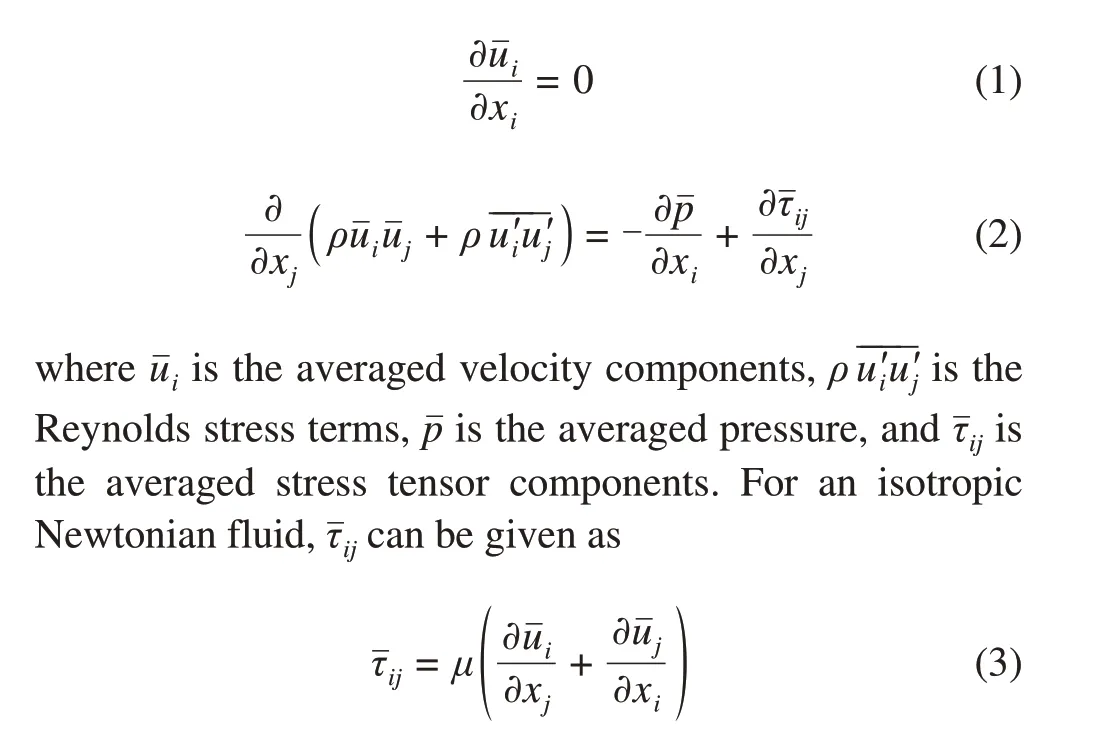
whereμis the dynamic viscosity of the fluid. In CFD,many techniques have been developed to model viscous turbulent flow fields. The selection of the correct turbulence model is of great importance for obtaining reliable results. In the simulations, two different turbulence models, shear stress transport (SST)k-ωand Reynolds stress model (RSM) are used for Reynolds stress terms. These models are two of the most common turbulence models for flow around ships(ITTC 2011).

The continuity, momentum, and turbulent transport equations are solved with a finite volume technique with a segregated algorithm (Wilcox 1994). A second-order upwind scheme is used for the discretization of the viscous terms, while a second-order central difference scheme is used for convective terms (Wilcox 1994). The pressure field is solved with the SIMPLE algorithm (Patankar and Spalding 1972).

3 Roughness function

The normalized mean velocity profile in the inner layer of a turbulent boundary layer can be expressed as(Clauser 1954)

whereU+is the normalized mean velocity,y+is the nondimensional normal distance from the wall,κis the von Karman constant,Bis another constant defined for the smooth surface, and ΔU+is the roughness function. ΔU+causes a downward parallel shift on the mean velocity profile, unlike on the smooth surface. In the analysis, the Griggson (1992) roughness function is used to model the roughness effects, as suggested by Unal (2015). The function is given as

wherek+is the roughness Reynolds number defined by Eq. (6), whereksis the characteristic roughness height,uτis the friction velocity, andνis the kinematic viscosity of the fluid.

4 Flat plate simulations

Flat plate simulations were performed using the same dimensions as the test bed dimensions of Unal (2015). The schematic of the test bed is shown in Figure 1.The roughness characteristics of 40-grit sandpaper are used for the sandpaper located in front of the test plate.

The experimental study (Unal 2015) was performed using nine different test specimens, including a smooth acrylic reference surface (coded as SM). Two different antifouling paints are used: a foul release solution (coded as AF1) and a self-polishing copolymer paint (coded as AF2). In the table, SP, RS, and RR indicate that the relative paint is applied with spraying, a smooth roller, and a rough roller, respectively.A blasted steel surface (BLA), a#40 grit (SAND40) sandpaper surface, and a #120 grit(SAND120)sandpaper surface are included in the scope of the study.

The roughness characteristics of the surfaces, measured with 50 mm cut-off lengths and 81-point window lengths,are shown in Table 1. In the table, Rt is the mean height between the highest peak and deepest valley, Ra is the mean deviation of the surface, and Rq is the root-meansquare deviation of the surface. Sk stands for skewness,Ku stands for kurtosis, and ES stands for the effective slope.The other parameters are the mean spacing between extremes(Sd1,Sd2,and Sd3)and mean spacing between zero-crossings(Sd4).

An important parameter for CFD simulation is to determine the characteristic roughness height (ks) of the surface, which depends on both the roughness characteristics and roughness function. The most effective and widely used way to determineksis regression analysis based on boundary layer measurements taken from flat plate experiments (Atlar et al. 2018). Unal (2015) gives the following highly accurate equation forks, which successfully represents all eight surfaces based on the Rq,Sk,and Sd4values of the surface.Figure 2.shows the roughness function correlation with Eq. (7) for all surfaces. Hence, characteristic roughness heights were calculated with Eq. (7), and the roughness functions were calculated with Eq.(5).

Figure 1 Schematics of the test bed(dimensions are in mm)(Unal 2015)

Table 1 Roughness characteristics of the surfaces(Unal 2015)

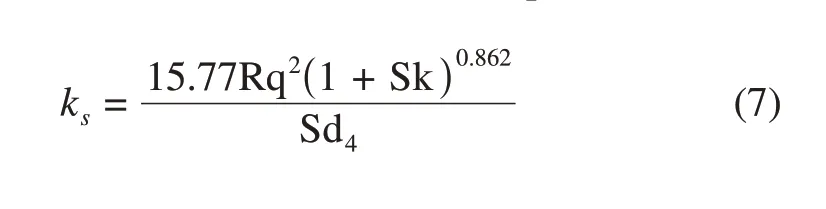
Figure 2 Roughness function correlation for all surfaces adopted from unal(2015)

Star-CCM+has a built-in roughness function that takes the roughness regime into consideration (CD ADAPCO 2011).However,Eq.(5)assumes that the flow is in either a transitional or fully rough regime. Implementation of Eq. (5) in the simulations is a technical issue that is addressed by setting low values for criticalk+values of hydraulically smooth and transitional regimes so that the flow is forced to be in a fully rough regime.This method was previously used and explained in detail by Demirel et al. (2014) and Karabulut et al.(2020).

A square prism-shaped computational model is used in simulations. The velocity inlet boundary condition is applied at the front edge of the plate, while the pressure outlet condition is applied at the rear edge. The rough wall boundary condition is applied for the sandpaper and test plate,while the smooth wall condition is applied for the remaining part of the test bed. Figure 3 shows the computational domain and boundary conditions for numerical analysis of the flat plate cases.

A trimmed hexahedral mesh was created using the builtin meshing tool of Star-CCM+. Near-wall refinement was achieved with prism layer meshes. The thickness of the first layer adjacent to the test bed was adjusted so that they+value of the cell centroid stayed in the log-law region of the boundary layer.Additional attention was given to keeping they+value of the adjacent cell centroid greater thank+, as suggested by CD-ADAPCO (2011). Figure 4 shows the longitudinal and top views of the generated mesh for the flat plate simulations.

Figure 3 Computational domain and boundary conditions

Figure 4 Mesh for flat plate simulations

To check the validity of the CFD methodology, friction velocities obtained from CFD and EFD are compared in Table 2. In the table,U∞is the free stream velocity, andk-ωand RSM indicate the results obtained using the SSTk-ωmodel and the RSM, respectively. The relative differences(RD)of theuτbetween CFD and EFD were calculated with Eq.(8).

The RDs of the results obtained with RSM were smaller than those of the results obtained with the SSTk-ωmodel for all cases except for the AF2_RS_6 case, for which the maximum RD of the RSM was 2.31%. The maximum RD for the results obtained with the SSTk-ωmodel was 5.49%,which occurred in the BLA_6 case.

Figure 5 shows the normalized mean velocity profiles of the smooth, SAND120, and SAND40 surfaces based on the inner variables of the boundary layers for a free stream velocity of 4 m/s.The smooth case closely follows the loglaw profile,while the velocity profiles of the rough surfaces shifted downward in accordance with the characteristic roughness height.

Figure 6 shows the mean velocities based on the outer variables of the boundary layer. In the figure,U∞is the free stream velocity andδis the boundary layer thickness.Boundary layer thickness is taken as the vertical distance at which the flow velocity in thexdirection is equal to99% of the free stream velocity. The figure shows thatu/U∞decreases for rough surfaces unlike with the smooth case. In addition, the decrease inu/U∞diminishes with increasingy/δ. This result is in good agreement with the experimental studies of Hama(1954).

Table 2 Comparison of the friction velocities

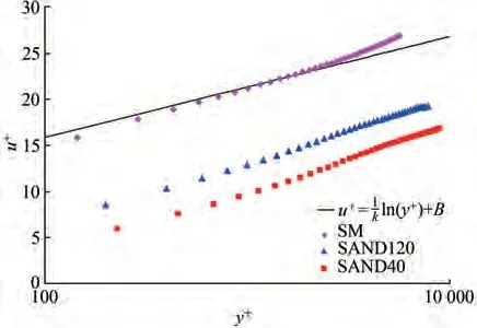
Figure 5 Mean velocity profiles with inner variables(U∞= 4 m/s)

Figure 6 Mean velocity profiles with outer variables(U∞= 4 m/s)

5 Simulations with surface ships

The flat plate simulation results show that the proposed methodology can be effectively used to investigate the roughness effects on the resistance characteristics of other geometries. Therefore, additional simulations were conducted with four different surface ship geometries using the same wall function approach. The ship geometries used in this study are Series 60 (CB= 0.6), KCS, a KVLCC2 tanker, and a navy combatant DTMB5415. Figure 7 shows the longitudinal views of the ships.The same model lengths (Lpp=15 m) were used in the simulations to compare the effect of roughness on different ship geometries at the same Reynolds number. All the ship simulations were performed atRe= 107.

Figure 7 Longitudinal view of the ships

The total resistance of a ship (RT) consists of several components: frictional resistance (RF) due to tangential fluid forces,viscous pressure resistance(RVP)due to threedimensional effects and wave resistance (RW) due to the loss of energy absorbed by waves.A useful approach is to non-dimensionalize these forces by using the density of the water (ρ), service speed (V), and wetted surface area(S) with Eq. (9) asCrepresents the relative non-dimensional resistance component.

The frictional resistance and the viscous pressure resistance of a ship are mainly caused by fluid viscosity. The main focus of this study is to investigate how these resistance components of different ship geometries are affected by different roughness conditions of its outer surface. Hence, free surface effects are simply ignored to obtain results much faster by using the steady model instead of the unsteady RANS model, which takes into account the free surface effects. Computational domains are limited to the still water surface.Velocity inlet boundary conditions were applied 2Lin front of the ships’ upstream end point,while pressure outlet conditions were applied 3Lbehind the ships’ downstream end points, whereLis the water length of the ship. Figure 8 shows the computational domain and boundary conditions for ship simulations.

Figure 8 Computational domain and boundary conditions for ship simulations

Similar to the flat plate analysis, computational meshes were created with the automated meshing tool of Star-CCM+.Figure 9 shows the created mesh for the KVLCC2 cases as an example. Several refinement zones are defined for the critical regions, such as near ship, bow and aft geometries, and wake zones. Near-wall refinements are achieved by prism layer meshes.

Figure 9 Volume mesh for KVLCC2 cases

A mesh convergence study was conducted using the Series 60 ship asks= 500 μm with the grid convergence index (GCI) method (Çelik et al. 2008). Three meshes were created by systematically changing the average cell sizes.Average cell sizes and the total number of cells are given in Table 3. Average wally+values calculated with RSM were also added to the table for comparison purposes.

Table 4 shows the GCI calculation results. The total number of the cells of meshes is represented byN.e21ais the approximate relative error of the fine mesh with respect to the medium mesh, andparepresents the apparentorder of the magnitude.Fine GCIs are calculated as 0.09%for the SSTk-ωmodel and 0.95% for the RSM, respectively.

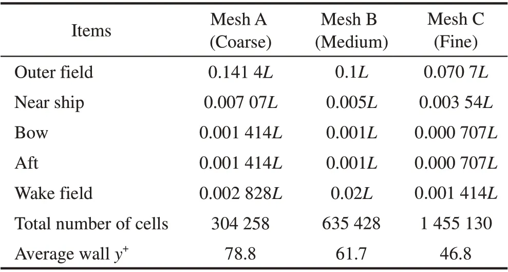
Table 3 Mesh characteristics for convergence studies

Table 4 Results of GCI calculation

On the basis of the results of the convergence study,fine mesh parameters were used for other geometries. Simulations were conducted for a wide range of surface conditions up toks= 500 μm.

Table 5 shows the calculated results for resistance coefficients. The increase in frictional resistance (ΔCF) and in viscous pressure resistance (ΔCVP) due to roughness were added to the table. The results of both turbulence models were in agreement for smooth cases(ks= 0),clearly showing that surface roughness has a direct effect on both frictional and viscous pressure resistance. The results of both turbulence models indicated that,as expected,frictional resistance increases with increasing surface roughness.However, the RSM provided a slightly greater resistance increase than the SSTk-ωmodel. Whenks= 500 μm, the resistance increase was calculated as 56.1% using the SSTk-ωmodel, while the increase was calculated as 66.1%with RSM.

Another significant difference was observed in viscous pressure resistance.The SSTk-ωmodel led to lowerCVPfor all surface conditions. In addition,CVPincreased with increasing roughness when the SSTk-ωmodel was used,while RSM achieved lowerCVPwhenks≤10 μm.Finally, a 44.1% increase inCVPwas observed with the SSTk-ωmodel, while this value was limited to only 21.4%with RSM.

Figure 10 compares theCFvalues of different ships,clearly showing that the geometry has a significant impact on the frictional resistance on rough surfaces.CFof smooth surfaces is around 0.003 for all ships. Whenks= 500 μm,CFof Series 60 ship and of KVLCC2 was 0.005 07 and 0.006 2, respectively. The most significant increase inCFwas observed on KVLCC2. DTMB 5415 has a similarCF-kscurve as KVLCC2, Series 60 has the lowest values,while theCF-kscurve of KCS is in between those of Series 60 and DTMB 5415.

Figure 10 Comparison of CF of ships for different roughness conditions(RSM)

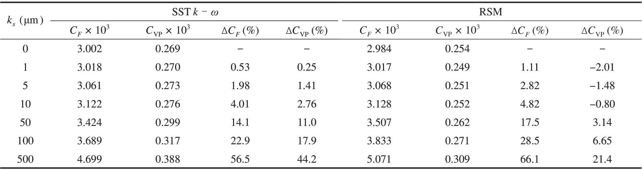
Table 5 Resistance coefficients of Series 60

Figure 11 shows the distribution of the local skin friction coefficient (cF) on the DTMB 5415 hull, and Figure 12 shows the distribution of the local skin friction coefficient on the Series 60 hull.From the figures,we can deduce that the frictional resistance of rough surfaces depends on the geometry of the bow. The bulbous bow geometry of the DTMB 5415 is the major reason for the greater frictional resistance increase of DTMB 5415 than that of Series 60.The local skin friction coefficient is calculated by using Eq.(10).Eq.(11),wherep-p∞is the dynamic pressure.The figure shows that the pressure at the aft portion of the hull is decreased due to the roughness, which results in increased viscous pressure resistance.

Figure 11 Distribution of skin friction coefficient on dtmb 5412 surface

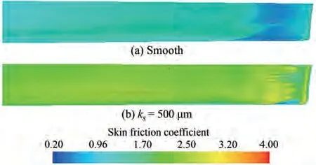
Figure 12 Distribution of skin friction coefficient on series 60 surface

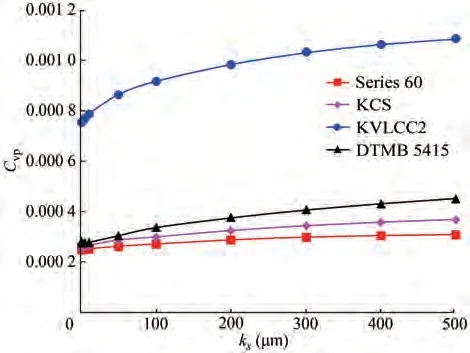
Figure 13 Comparison of CVP of ships for different roughness conditions(RSM)

Figure 14 Dynamic pressure coefficient distribution on the kcs hull

The effect of roughness on pressure distribution becomes clearer when the velocity field is investigated. The velocity distribution (normalized by the service speed)behind KCS is shown in Figure 15. The velocity at the stern of the ship decreases as a result of surface roughness.The wake field becomes larger due to the decrease in velocities,and hence,the pressure behind the hull decreases.

Figure 16 shows the streamwise normalized velocity distribution in the boundary layer around the KCS hull for various sections. The roughness on the surface causes a significant increase in the thickness of the boundary layer.The velocity around the hull decreased,and the viscous effects became more dominant due to roughness.

Figure 17 shows the pressure distribution around the water level of the KCS hull. No significant difference in pressure is found due to the roughness in the parallel body of the vessel.However,the pressure at the stern of the vessel decreases for the rough case,which results in increased viscous pressure resistance.

Figure15 StreamwiseVelocityDistributionBehind KCS at y=0.005 Lpp

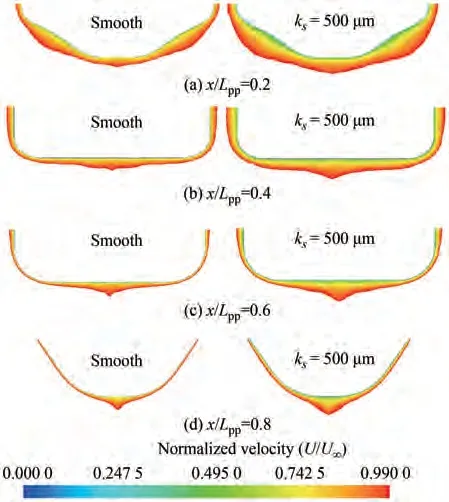
Figure 16 Streamwise velocity distributions around KCS hull. Velocities are limited to U = 0.99 U∞depicting the boundary layer

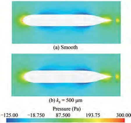
Figure 17 Pressure distribution at water level around the KCS Hull

6 Conclusions

In this study, the effect of hull roughness on the viscous resistance characteristics is investigated using a RANSbased approach. The wall function is modified with the roughness function model in accordance with the EFD data of Unal(2015).

Validation studies were performed by comparing the friction velocities of the CFD results with the EFD data of Unal (2015). The maximum relative error of the SSTk-ωmodel was 5.49%, while the maximum relative error of the RSM was 2.31%when compared with the experimental results. Grid convergence studies were performed using Series 60 geometry with three meshes that have different resolutions. Results of the GCI method indicated that the mesh characteristics of the fine mesh are sufficient for further calculations.

Simulations were conducted with four different surface ship geometries. The behavior of the frictional resistances was significantly different for different ship types.An examination of the distributions of the local skin friction coefficients of the DTMB 5415 and Series 60 showed that the plumpness of the bow form has a significant effect on the increase in frictional resistance with increasing roughness. Another significant finding of the study is that viscous pressure resistance is directly affected by the surface roughness. For all geometries, viscous pressure resistances showed a significant increase for highly rough surfaces.

Discrepancies were found between the predictions of the RSM and the SSTk-ωmodel for the viscous pressure resistances of the slightly rough surfaces. In all simulations with the SSTk-ωmodel, viscous pressure resistances increased with increasing roughness, whereas some simulations with the RSM predicted small decreases in viscous pressure resistance.

Another important topic is the scale effects on the roughness. In addition, free surface effects are not covered in this study. The authors intend to cover these points in their future studies.

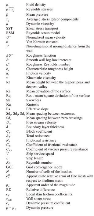
Nomenclature