On the decay and regularity of the strong solution to the 2D MHD equations in a strip domain
2022-08-02GuiGuilongLiYancanLiZilai
Gui Guilong ,Li Yancan ,Li Zilai
(1.School of Mathematics,Northwest University,Xi′an 710127,China;2.School of Mathematics and Information Science,Henan Polytechnic University,Jiaozuo 454003,China)
Abstract:We investigate in this paper the initial boundary value problem of the twodimensional incompressible magnetohydrodynamic system without magnetic diffusion in a strip domain.Making use of the explicit solution to the linear problem of perturbations system around the equilibrium,we established the linear decay of the strong solutions to the linearized system around the equilibrium state(0,e2)with the Navier-type boundary condition on the velocity.Moreover,the H3-regularity of the global strong solutions to the system is obtained by using anisotropic Sobolev technique.
Keywords:the magnetohydrodynamic equations,linear decay,regularity
1 Introduction
We consider in the paper the two-dimensional incompressible magnetohydrodynamic(MHD)equations without magnetic diffusion with the Navier-type slip boundary conditions


Hereu=(u1,u2)Tis the velocity field,B=(B1,B2)Tis the magnetic field,pis the pressure,and Ω is a strip domain in R2:

The system(1)can be applied to model plasmas when the plasmas are strongly collisional,or the resistivity due to these collisions are extremely small.For the relevant physical background of this system,one can refer to[1]and the references therein.As we know,the 2D MHD equation with magnetic diffusion has a global smooth solution,see[2-3].Recently,the global well-posedness and stability problem of the 2D MHD equations without magnetic diffusion have attracted the attention of many mathematicians.
For the 3D case,Abidi and Zhang[4]proved the global well-posedness of the Cauchy problem of the 3D incompressible MHD system with initial data close enough to the equilibrium state(0,e3),and in the case when the initial magnetic field is a constant vector,they also obtained that the large time decay rate of the solution.And there are some result about global small solutions to this system in[5-7].For the 2D case,Ren,Wu,Xiang and Zhang[8]proved the global existence and the decay estimates of small smooth solution for the 2-D MHD equations without magnetic diffusion in the whole space,and this confirms the numerical observation that the energy of the MHD equations is dissipated at a rate independent of the ohmic resistivity.And for the 2D system(1)around the equilibrium state(0,e2),there are some results about global small solutions to the incompressible MHD system in[9-11],and in particular,Ren,Xiang,and Zhang[11]proved theH2global well-posedness of the system under non-slip boundary conditions and Navier-type slip boundary conditions respectively in a strip domain.
We focus in the paper on small perturbations of the system(1)around the equilibrium state=(0,e2)withe2=(0,1)T∈R2.Notice that the boundary conditions(2)mean

we thus setb:=B-e2and reformulate the system(1)-(2)as follows

Based on the result in[11],we will study the linear decay and theH3regularity of the global solution of the system(5).
The first result is the decay to the solutions of the 2D linear MHD equations without magnetic diffusion in a strip domain.

By eliminating the variablebin(6),we can get theuequations

whereu1(x)=ut(x,0)andut(x,0)is given by(12).We will first obtain the explicit solutions of the linear equations(7)by separating variables method from[12-13],and then directly calculate the decay of the solutions.
Theorem 1.1Assumem0∈N+,Then the linear system(6)has a unique solution(u,b)satisfying

and for somer>0,

Remark 1.1By eliminating the variableuin(6),we can also get thebequations which has the same form as(7),and we thus get the same decay ofbasu.
The second result is aboutH3-regularity of the solutions of the 2D MHD system(5).Since∇·Δu=0 in Ω and

we have

First,taking Helmholtz projection P to equation(5)1,we have

Form∈N,we define the energiesand the dissipationsby

and

Motivated by[11]and[14],we will get theH3regularity of the global strong solution to the 2D MHD system(5).
Theorem 1.2Let(u0,b0)∈H3(Ω)satisfy

and compatibility conditions

andp(0)is determined by

Then there exists a small positive constantϵ0such that if

then the MHD system(5)admits a unique global solution(u,b)∈C([0,+∞);H3(Ω)).Moreover,there exists a positive constantCsuch that for anyt>0,

Remark 1.2Ifon∂Ω,according to(11)2and the Navier-type slip boundary conditions(2),we have∂1b2=0 on∂Ω.
Remark 1.3The main difficulty of improving the regularity of the global solution onHm(m≥3)lies in the improvement of the order of the normal directional derivative.In fact,according to the method in this paper,we can continue to improve the normal regularity of the solution and keep the order of the normal derivative of the solution the same as that of the horizontal derivative.
The rest of the paper is organized as follows.Section 2 introduces the main lemmas used in this paper.In section 3,by making use of the explicit solution to the linear system(7),we prove Theorem 1.1.Finally,we establish the global uniform a prioriH3estimates for the system(5)and complete the proof of Theorem 1.2 in Section 4.
Notation 1.1Let us end this introduction by some notations that will be used in all that follows.
Fora≾b,we mean that there exists a uniform constantC,which may be different on different lines,such thata≤Cb.Fora~b,we mean thata≾bandb≾a.For operatorsAandB,we denote[A,B]=AB-BAthe commutator ofAandB.Fors∈R,we define the operatora pseudo-differential operator with the symbol〈ξ2〉s(or|ξ2|s),that iswhereF(orF-1)is the Fourier(or inverse Fourier)transform[12]operator and.We also denote aboveFby^for simplicity.Throughout the paper,the subscript notation for vectors and tensors as well as the Einstein summation convention has been adopted unless otherwise specified.
2 Preliminaries
Let us introduce Sturm-Liouville problem and recall some properties of Sturm-Liouville problem which will be used in the Section 3.

whereαi,βi≥0,αi+βi>0 andi=1,2.The problem of finding an eigenvalueλsuch that equation(16)has a non-zero solution is called Sturm-Liouville problem,and the non-zero solutionXλcorresponding to the eigenvalueλis called the eigenvector of the eigenvalueλ.
Lemma 2.1[13](Some properties of Sturm-Liouville problem)For Sturm-Liouville problem(16),there are the following properties:
(1)For the eigenvalueλ,there holdsλ≥0.In particular,ifβ1+β2>0,thenλ>0.
(2)For the eigenvalueλandμ,ifλ/=μ,then
Then,let us recall some basic estimates,which will be heavily used in section 4.
Lemma 2.2[15](classical product laws in Sobolev spaces)Fork>0,there holds

Lemma 2.3[15]Fork≥1,there holds

Lemma 2.4[14]Let Ω be the strip domain defined by(3),then there exists a positive constantC=C(Ω)such that

for anyu=(u1,u2)T∈H2(Ω).
Lemma 2.5[11]Let Ω be the strip domain defined by(3),then there exists a positive constantCsuch that

for anyu=(u1,u2)T∈H2(Ω)with∇·u=0 in Ω andu1=0 on∂Ω.
Lemma 2.6[17](Poincar´e′s inequality)Let Ω be the strip domain defined by(3).AssumeU⊂Ω,then for all

Lemma 2.7[15,18](the Helmholtz Decomposition inHm(Ω))Let Ω be the strip domain defined by(3),every vector fieldu∈Hm(Ω)(m∈N),has the unique orthogonal decompositionu=w+∇φ,where,∇φ∈Hm(Ω),w=Pu,and P is the Helmholtz projection which is defined byP:where

For the Stokes system

we have the following lemma about Stokes estimates.
Lemma 2.8[11]Let Ω be the strip domain defined by(3)andf∈Hm(Ω)form≥0.Ifu∈H1(Ω)is a weak solution to the system(19)withu1=∂1u2=0 on∂Ω,thenu∈Hm+2(Ω)and

Let′s recall the local well-posedness of the system(5)in[11]as follows.
Lemma 2.9[11](local well-posedness)Assume that the initial data(u0,b0)∈Hm(Ω)(m≥2)such that∇·u0=∇·b0=0 in Ω,u1=∂1u2=b1=∂1b2=0 on∂Ω,then there exists aT>0 such that the MHD system(5)admits a unique solution(u,b)on[0,T]satisfying(u,b)∈C([0,T];Hm(Ω)).
3 Proof of Theorem 1.1
From the basic theory of linear partial differential equations[19],we know that the linear system(6)has a unique solution(u,b)satisfying(8).So we need only to prove(9).For this,we will split the proof into the following two steps.
Step 1Explicit solutions
By the Fourier transform with respect to the horizontal variablesx2∈R corresponding Fourier variablesξ2∈R,the linear problem(7)translates to the following linear problem:

We will solve the above linear problem(21)by applying the separated variable method.
First,we consider nonzero solutions in the form of separated variables,that is,forwith

whereTi(t)=Ti(t,ξ2)andXi(x1)=Xi(x1,ξ2)will be determined later on.
Combining the first equation of(21)with(22),we have

that is

Therefore,we have

Combining the second equation of(21)with(22),we obtain that


From(23)and(25),we get the following Sturm-Liouville problem

Our goal is to find the eigenvalueλi(ξ2)that makes the Sturm-Liouville problem(26)have a non-zero solution.
In fact,thanks to Lemma 2.1,we know thatλi(ξ2)>0.Then back to(23),we know that its general solutions are

whereare undetermined constants.Combining(27)with(25),we prove

Ifthere would beX1≡0 orX2≡0.This contradicts with the fact that^ui/≡0,so

From this,we find all eigenvalueswithi=1,2,n=1,2,3,···and the eigenfunctions corresponding to eigenvaluesandin(26)as follows


whereAi,n(ξ2)andBi,n(ξ2)are undetermined coefficients(which will be solved according to the initial data),and

Therefore,we get the solutions of(21)in the form of separated variables as follows

Thanks to the principle of linear superposition,we find that the solutionsinof(21)have the forms

In particular,for the initial data

thanks to the third equations in(21),we obtain that the coefficientsAi,nandBi,nsatisfy

which determines coefficientsAi,nandBi,n.

Step 2Linear decay


Let′s estimateIn fact,fromwe get


Thanks to(31),we have

then forJ111,there holds

which implies

wherer1=r1(ℓ)is a positive constant.

wherer2=r2(ℓ)is a positive constant.Forξ2∈D,one has D≥0,which implies

ForJ121,there holds


ForJ122,there holds

ForJ2,we split it into two parts,

Similar toJ121andJ122,we have

and

whereCis a suitable positive real numbers.
Combining the above estimates with(32),we have

which implies

Similarly,we may get

This ends the proof of Theorem 1.1.
4 Global well-posedness in H3(Ω)
In this section,we follow the ideas in[11]and[14]to get the solution of system(5)inH3.Notice that in the strip domain Ω,there holds[∂2,P]=0 but[∂1,P]0 in general.In order to high regularities of the solution of system(5),we first prove the following proposition.
Proposition 4.1Letf∈H3(Ω)satisfyingf1=0 on∂Ω and(Ω),then

ProofBy a simple density argument,it is needed only to show the desired results are valid whenfandgare smooth enough.Thanks to Lemma 2.7,we may findφ∈H2(Ω)such that

with P(f·∇f)·n=0 on∂Ω.Notice that|(f·∇f)·n|=|f1∂1f1+f2∂2f1|=0 on∂Ω,then we get|∂1φ|=|∇φ·n|=0 on∂Ω.Hence,one has

which complete the proof of Proposition 4.1.
We are now in a position to prove Theorem 1.2.
Proof of Theorem 1.2Based on Lemma 2.9 and the global well-posedness result of system(5)inH2(Ω)in[11],we need only to give uniformly a priori estimates inH3(Ω).Toward this,we split it into 12 steps.
Step 1Estimate of
By taking theL2inner product of equations(11)1and(11)2withuandbrespectively,and integrating by parts,we readily obtain

Step 2Estimate of
We take the horizontal derivative(k≤m)of equations(11)1and(11)2,and then takeL2inner product of them withandrespectively.Summing them over 1≤k≤m,we obtain


Thanks to Lemma 2.2 and H¨older′s inequality,we get

Similarly,thanks to Lemma 2.3,one has

ForI2+I4,due to the fact thatwe prove

ForI21,there holds

And forI22,one finds

Substituting the estimate ofI1,I2,I3andI4into(34),we have

Step 3Estimates of
We apply the horizontal derivative operatorsto equations(11)1and(11)2,and then take theL2inner product of them withandrespectively.Summing them over 1≤k≤m,we deduce that

Thanks to Lemma 2.2 and H¨older′s inequality,we have

Similarly,there holds

On the other hand,forII2,we splitII2into three parts.

We estimateII11andII13by

and

While thanks to Poincar´e′s inequality,one obtains

ForII3,we split it into three parts,

Similar toII11andII12,we get

SubstitutingII1,II2,II3andII4into(36),we obtain

Step 4Estimate of
We apply the horizontal derivative operatorsto equations(11)1and(11)2,and then take theL2inner product of them withrespectively.Summing them over 1≤k≤m,we find that

Thanks to Lemma 2.2 and H¨older′s inequality,we have

and

And thanks to Poincar´e′s inequality,there holds

and

Therefore,we obtain

Step 5Estimate of
Thanks to divergence-free conditions ofuandb,we find

which are bounded by Steps 1 and 2.Hence,we need only to estimate

Toward this,we introduceωandβ,where

Acting curl to equations(5)gives rise to
Notice that

and

Then combining Step 1 and Step 2,we know that the estimate of

implies the estimate of

By taking theL2inner product of equations(40)1and(40)2ofωandβrespectively,and integrating by parts,we obtain

Now,let′s deal with the casek≥2.We take the horizontal derivative operatorsto equations(40)1and(40)2,and then theL2inner product withandrespectively.Summing them over 2≤k≤m,we deduce that

Whenk=2,according to H¨older′s inequality,we get

and

And forIV2andIV4,since

there holds

Whenk≥3,we estimateIV1andIV3by

and

ForIV2andIV4,thanks to Lemma 2.3,there holds

Combining the above estimates in this step,we prove

Step 6Estimate of
We take the horizontal derivative operatorsand the time derivative∂tof equations(11)1,and then take theL2inner product of them withBy integration by parts,we find that

where 2≤k≤m.For the case ofk=2,we haveV2=0 and

Let′s now deal with the casek≥3.Thanks to Lemma 2.2,one can see

And thanks to Lemma 2.3,forV2,we find

ForV4,by integration by parts and due to∇·b=0,we obtain

then according to Lemma 2.2,we get

Combining the above estimates in this step,we prove

Step 7Estimate of
Similar to the proof in Step 5,we may get

and


Fork=2,there hold

and

Thanks to Poincar´e′s inequality,we may get

and

Whenk≥3,we estimateV I1andV I4by

and

Thanks to Poincar´e′s inequality again,one can see that
and

Combining all estimates above,we obtain

The above estimates are mainly about the horizontal derivatives ofuandband some about the vertical derivatives ofuandb.In order to close the energy estimate form=3,we need more estimates of the vertical derivatives ofuandb.
Step 8Estimate of
Applying the time derivative∂tto the first equation of(40)and taking theL2inner product withωtyield

Noticing thatV II2=0 and similar to estimates in Step 7,we get

Here,substitutingV II1,V II2,V II3andV II4into(45),we have

Step 9Estimate of

where 2≤l≤k≤m.
Sinceb1=∂1b2=0 on∂Ω and∇·b=0 on∂Ω,forl=2,we find

and forl=3,one can see


Combining(47)with(48),one has

For the case of(l,k)=(2,3),we estimateV III1andV III2by

and

And forV III3andV III4,one finds

and

Combining the estimates ofV III1,V III2,V III3,andV III4with(49),we obtain

For the casel=k=2,we first boundV III1by

And forV III2,we split it into three parts,

Due to∇·b=0,we readily get

While thanks to Lemma 2.5,one can see

which along with(51)implies

SetWe splitV III3into five parts,Due to∂1u1=-∂2u2,there holds


Similarly,we get

Hence,one obtains

Next,we splitV III4into seven terms,

Applying H¨older′s inequality yields

and

which along with the decomposition ofV III4above implies

Therefore,for the casel=k=2,combining the estimates ofV III1,V III2,V III3,andV III4with(49),we can obtain

Finally,we consider the casel=k=3.
Thanks to Proposition 4.1,we have

Sinceu1=b1=∂1u2=∂1b2=0 on∂Ω,there holds

which follows

ForV III2,we split it into two parts,

Thanks to∂1b1=-∂2b2,one can see

While due to Lemma 2.5,we have

Next,let′s estimateV III3.Noticing that(u·∇∂1Δb,∂1Δb)L2=0,we splitV III3into four parts,

SetWe have

Integrating by parts leads to

Applying H¨older′s inequality yields

Then,forV III3,we get

Similarly,forV III4,one finds

We splitV III41into four parts,
It follows from integration by parts that

and

Applying H¨older′s inequality again yields

Hence,forV III4,we prove

Therefore,for the casel=k=3,combining the estimates ofV III1,V III2,V III3,andV III4with(49),we obtain

Step 10Estimate ofV1andV2(m=2,3)
In Step 9,V1andV2cannot be estimated directly by using integration by part.We overcome this difficulty with the help of the method in[2].Firstly,using the equation(11)2,we can get

and using the equation(11)2again,we have

Combining(55)with(56),we may get

Thanks to the first equation in(5),one can see

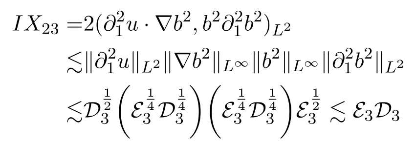
Due tou1=b1=∂1u2=∂1b2=0 on∂Ω and by(58),we have=0 on∂Ω.Next,forIX1,by integration by parts,we have

ForIX2,we first split it into three parts,

We also find that
SetOne can see that

ForIX24,it follows

ForIX23,ifm=2,thanks to Lemma 2.5,there holds
and ifm=3,one can see

Hence,combining the estimates ofIX21,IX22andIX23,we obtain

Similarly,forIX4andIX5,we also have

Substituting(59)-(61)into(57)yields

We use repeatedly the second equation in(11)to obtain
which implies
Next,let us estimateIX31andIX32,thanks to Lemma 2.4 and Lemma 2.5,there holds
Ifm=2,similar toIX31,we estimateIX32by
and ifm=3,we splitIX32into three parts,

Similar toIX31,forIX321andIX322,there holds

Finally,forIX323,integrating by parts yields

Therefore,we obtain

Combining(62)and(64)leads to

WriteCombine(53)and(54)with(65)respectively,so we can eliminateV1andV2respectively to obtain

and

Step 11Estimate ofwith 2≤l≤k≤3
In this step,we will estimate(2≤l≤k≤3)by Stokes estimates.From(5),we may find the equations ofuas follows,

According to Lemma 2.8,we have

wherem=2,3.
Whenm=2 in(68),one has

which implies

Due to∇·b=0 and Lemma 2.5,we have

Form=3 in(68),it follows from(70)that

which gives rise to

Step 12Closing a priori estimates
Thanks to the local well-posedness result(Lemma 2.9),there exists a positive timeTsuch that the system(5)with initial data(u0,b0)∈H3(Ω)has a unique solution(u,b)∈C([0,T);H3(Ω))).
Set

where the small constantc0will be determined later on.We will combine the estimates in Steps 1 to 11 to close a priori estimates.
In fact,for anyt∈[0,T*),it follows from(69)and(71)that

Hence,ifc0satisfies

then there holds

On the other hand,we takem=3 in Steps 2 to 7 and set

and
According to∇·u=0 and∇·b=0,we know that

For any given small positive constantσ1,we set

and

From this,we find that there is a small enoughσ1>0 such that the following inequalities hold

for some suitably small positive constantc1.
Similarly,for any given small positive constantσ2,we set

and

By these definitions,we find that there is a small enoughσ2>0 such that the following inequalities hold

for some suitably small positive constantc2.
Combining(81)with(33),(35),(37),(39),(41)-(43),we obtain

While combining(84)with(50),(66),(44),(46)and(67),one has

which along with(85)ensures

and then

for some positive constantC3≥1,wherec3:=min{c1,c2}.
Therefore,we deduce from(78),(87),and(75)that

Hence,ifc0satisfies

then there holds

Integrating(90)onτ∈[0,t]yields

According to compatibility conditions(12)and(13),one has

for some positive constantC4≥1,and we thus obtain

provided

Combining(91),(92)with Stokes estimates(75)in Step 11 ensures that there exist a small positive constantc4and some constantC6≥1 such that

which along with(78)implies

for some constantC7≥1.
Therefore,due to(74),(89),(93),for any given

we get(95).So,we takeϵ0in(14)such thatto obtain

which follows from(72)thatT*=+∞,and then finishes the proof of the global well-posedness part.
Thanks to(91)and(75),we obtain,for some positive constantsc5andC8,

that is

This ends the proof of Theorem 1.2.
