Yuan Gong(公元) and Wen-Xing Zhu(朱文兴)

School of Control Science and Engineering,Shandong University,Jinan 250061,China

With the increasing maturity of automatic driving technology, the homogeneous traffic flow will gradually evolve into the heterogeneous traffic flow,which consists of human-driving and autonomous vehicles. To better study the characteristics of the heterogeneous traffic system, this paper proposes a new car-following model for autonomous vehicles and heterogeneous traffic flow, which considers the self-stabilizing effect of vehicles. Through linear and nonlinear methods,this paper deduces and analyzes the stability of such a car-following model with the self-stabilizing effect. Finally, the model is verified by numerical simulation. Numerical results show that the self-stabilizing effect can make the heterogeneous traffic flow more stable,and that increasing the self-stabilizing coefficient or historical time length can strengthen the stability of heterogeneous traffic flow and alleviate traffic congestion effectively. In addition,the heterogeneous traffic flow can also be stabilized with a higher proportion of autonomous vehicles.

Keywords: heterogeneous traffic flow,self-stabilizing effect,car-following model,autonomous vehicle

1. Introduction

Nowadays, the increasing number of cars has caused a series of problems such as traffic congestion and environmental pollution. The intelligent transportation system (ITS)aims to improve traffic efficiency,suppress traffic congestion,and reduce pollution. As a typical microscopic traffic flow model, the car-following model is widely used to investigate the driving behavior in the ITS environment. The classical car-following model was first proposed by Pipes[1]in 1953. In 1995,Bandoet al.[2]improved Pipes’model and proposed the optimal velocity model(OVM).Nagatani[3]and Sawada[4]analyzed the traffic flow by nonlinear methods and found that the interaction of the next-nearest-neighbor can enhance the stability of traffic flow.Jianget al.[5]constructed the full velocity difference model(FVDM),which considers both positive and negative velocity differences. Later, many scholars improved the traditional car-following model by incorporating different factors.[6–29]Geet al.[6]extended the optimal velocity model by combining the effect of backward looking with the ITS environment. Liet al.[13,14]introduced the self-stabilizing control into the OVM and proved that traffic stability can be significantly strengthened via self-stabilizing control. Chenet al.[19]improved the car-following model by considering the expected effect and self-stabilizing effect. Peng[25]studied the relationship between traffic interruption probability and traffic flow stability based on an extended optimal velocity model.

In recent years,with the fast development of intelligence and automation, autonomous vehicles have attracted many researchers’ attention.[30–34]Homogeneous traffic flow will gradually evolve into heterogeneous traffic flow in the next few years. To enable autonomous vehicles to drive cooperatively with human-driving vehicles, many scholars have carried out certain studies on the characteristics of the heterogeneous traffic system.[35–49]Zhuet al.[37]proposed a car-following model with adjustable sensitivity and smoothing factor, and used it to investigate the mixed traffic flow. Xieet al.[40]modeled heterogeneous traffic through a general car-following model framework,and demonstrated that connected vehicles play an important role in improving traffic efficiency. Anet al.[42]put forward a car-following model with the discrete following interval for autonomous vehicles,and discussed the impact of discrete car-following interval on stabilizing mixed traffic flow. Wanget al.[43]researched the mixed traffic system from the aspects of controllability theory and optimal controller design. These studies analyzed the properties of heterogeneous traffic flow from different perspectives. However,most existing studies did not fully consider the effect of self-stabilizing in heterogeneous traffic flow. Therefore, this paper incorporates the self-stabilizing effect into the car-following model for heterogeneous traffic flow and proposes an improved carfollowing model, which enables the vehicle to use the information of both its own and other vehicles to jointly control its driving behavior.

The paper is organized as follows. Section 2 proposes a new car-following model for heterogeneous traffic flow. Section 3 gives the linear stability condition of the proposed model by linear stability analysis. Section 4 gives the mKdV equation and the kink-antikink solution of the model by nonlinear analysis. Section 5 conducts numerical simulations to verify the theoretical results. Finally,Section 6 concludes this paper.

2. Models

Figure 1 shows a heterogeneous traffic system mixed with human-driving and autonomous vehicles (human-driving vehicles are green and autonomous vehicles are orange). In this system,Nvehicles distribute on a single-lane road without overtaking.

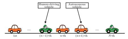
Fig.1. The illustration of the heterogeneous traffic system with N vehicles.

2.1. Model for human-driving vehicles

The dynamic model for human-driving vehicles is constructed based on Bando’s optimal velocity model(OVM)[2]

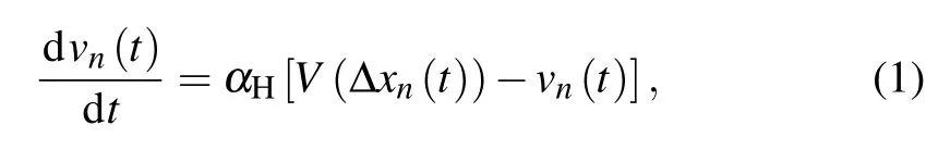
whereαH=1/τHis the driver’s sensitivity coefficient,τHis the driver’s reaction time;vn(t)is the velocity of vehiclenat timet; Δxn(t)=xn+1(t)−xn(t) is the headway between vehiclenand vehiclen+1 at timet;V(Δxn(t)) is the optimal velocity function(OVF).

Based on the OVM,Liet al.[13]proposed an extended carfollowing model with the self-stabilizing effect,which considers the velocity of the vehicle at a historical time. It is formulated as

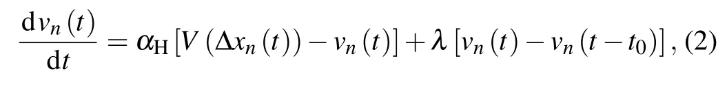
wherevn(t −t0) is the velocity of vehiclenat the historical timet −t0;vn(t)−vn(t −t0)is the self-stabilizing term,which means the difference between the current velocityvn(t) and the historical velocityvn(t −t0);λis the control coefficient.

Furtherly, Chenet al.[50]considered the continuous change of vehicle velocity in a historical time period,and presented a modified car-following model:

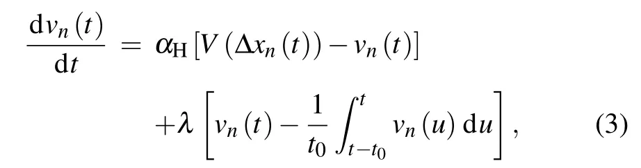
wheret0is the historical time length;dudenotes the average velocity of vehiclenat time [t −t0,t], which can describe the continuous velocity change of the vehicle in a historical time period;ducan be regarded as an extended self-stabilizing term,which represents the difference between the velocity of vehiclenat timetand its average velocity at time[t −t0,t];λis the self-stabilizing coefficient.

In Chen’s model,[50]the velocity of a vehicle in a historical period is taken into account in the effect of selfstabilizing, so the vehicle information can be utilized more sufficiently.Therefore,this paper uses Chen’s model[50]as the car-following model for human-driving vehicles. The optimal velocity function is given as[51]

wherevmaxrepresents the maximum velocity andlndenotes the length of vehiclen. Furthermore,due to the heterogeneity of different drivers in real traffic, the sensitivityαHcan take different values for different drivers.

2.2. Model for autonomous vehicles

Autonomous vehicles can obtain information from other vehicles through sensors,such as the position and velocity of the front and back vehicles. Recently,Zhuet al.[37]proposed a new car-following model for autonomous vehicles by incorporating the backward headway into the OVM:

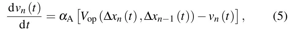
whereαArepresents the sensitivity of the autonomous vehicle,andVop(Δxn(t),Δxn−1(t))is the generalized optimal velocity function:

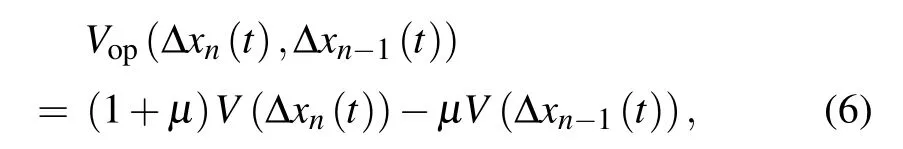
whereµ ∈(0,0.5)is the smooth factor,and the expression ofV(Δxn(t))is the same as that in Eq.(4).

Similar to the model for human-driving vehicles (3), the autonomous vehicle can also use the position or velocity of the vehicle itself in the historical time period to realize selfstabilizing control. Then the autonomous vehicle can use the information of the current vehicle itself and other vehicles simultaneously during its driving process. Therefore, to better describe the driving behavior of autonomous vehicles, a newcar-following model with the self-stabilizing effect is established as follows:

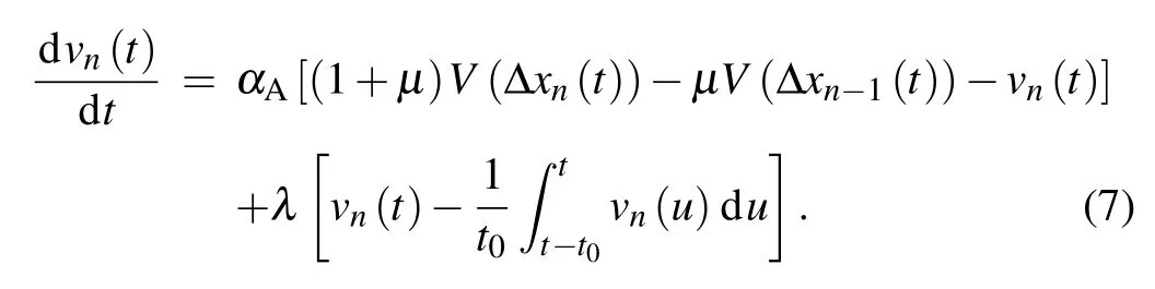
Here,we assume that the self-stabilizing effect of autonomous vehicles has the same form as that of human-driving vehicles.The meaning of the parameters in Eq. (7) is the same as that in Eqs.(3)and(5). Whenλ=0, the proposed model(7)reduces to model (5), which represents the model without selfstabilizing effect; whent0→0, fromdu=vn(t)we can obtain that model(7)also reduces to model(5).

2.3. A generic model for heterogeneous traffic flow

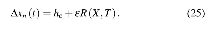
By comparing the equations of models (3) and (7), the two models can be rewritten into a unified form

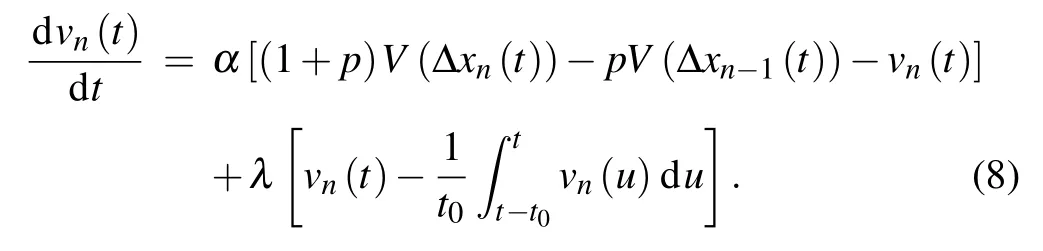
In this equation,αis the sensitivity of the vehicle, and the sensitivity of autonomous vehiclesαAis higher than that of human-driving vehiclesαH;pis the interaction coefficient between the current vehicle and the back vehicle. For autonomous vehicles,the interaction coefficientpis the smooth factorµ(see Subsection 2.2);for human-driving vehicles,the backward headway is not considered during driving, sopis equal to zero. Therefore,the interaction coefficientpis taken as

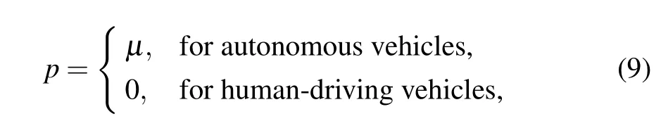
where 0<µ <0.5.

3. Linear stability analysis

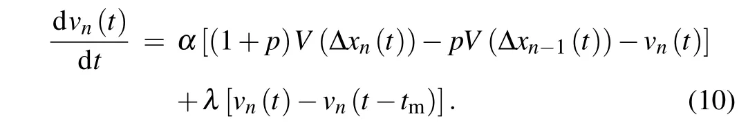
In this section, the linear stability analysis of the proposed model is conducted. First, according to the mean value theorem of integrals, there existstm∈[0,t0] such that. Then the proposed model(8)is reformulated as follows:

Furtherly,we can derive the following formula by performing the first-order Taylor expansion onvn(t −tm):

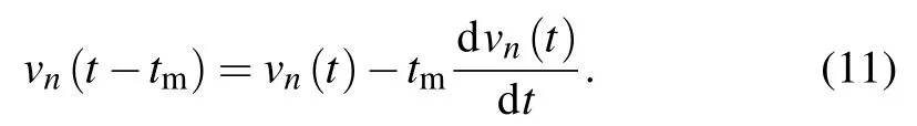
If equation (11) is substituted into Eq. (10), the following equation can be deduced:

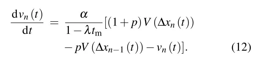
Letαm=α/(1−λtm),and then equation(12)can be rewritten into the following form:

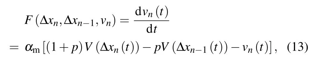
whereF(Δxn,Δxn−1,vn)is the acceleration function.

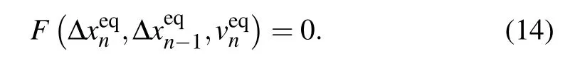
When the traffic flow reaches a steady-state equilibrium,the headway and velocity of vehicles are given by Δxn(t)=,and. Then the traffic flow in a steady state must satisfy the following equation:

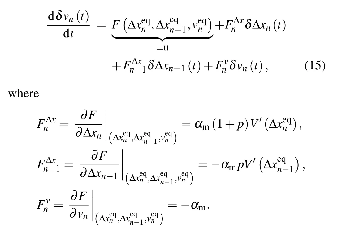
Add a small disturbance to the steady-state solution: Δxn(t)=,andvn(t)=. Inserting them into Eq.(13)and conducting the first-order Taylor expansion, we can derive the following linearized equation:

Suppose thatδΔxn(t) = ΔXnexp(iωn+st),δΔxn−1(t) =ΔXn−1exp{iω(n−1)+st}, andδvn(t) =Vnexp(iωn+st),where ΔXn, ΔXn−1, andVnare constants. According to Δxn(t) =xn+1(t)−xn(t) and, we can get

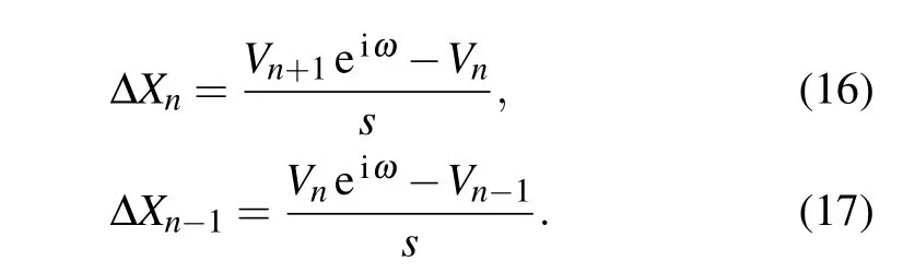
Incorporating Eqs.(16)and(17)into Eq.(15),we can obtain the following equation:

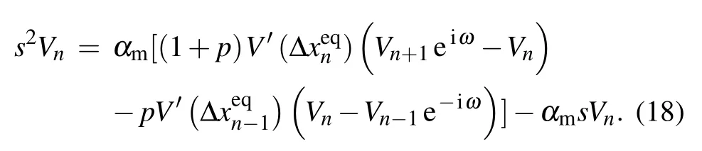
Now let us consider the case of uniform traffic flow,where all vehicles have the same steady-state velocity and the same equilibrium headway. ThenVn=Vn+1=Vn−1and,and then we can reduce Eq.(18)to a simplified form

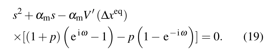
Assume that the solution of Eq. (19) has the following form:s=s1(iω)+s2(iω)2+···. After substituting it into Eq.(19)and ignoring the higher-order terms,we can solve the first-and second-order terms of iω:

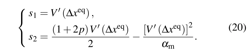
The necessary condition for a stable uniform traffic flow is Re(s)<0,i.e.,

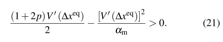
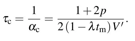
By solving the above inequality and consideringαm=α/(1−λtm),the linear stability condition of the uniform traffic flow is derived as follows:

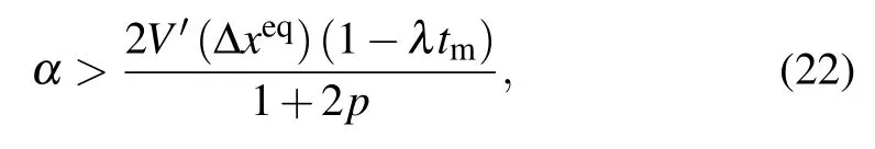
where the prerequisiteλtm<1 must be satisfied.

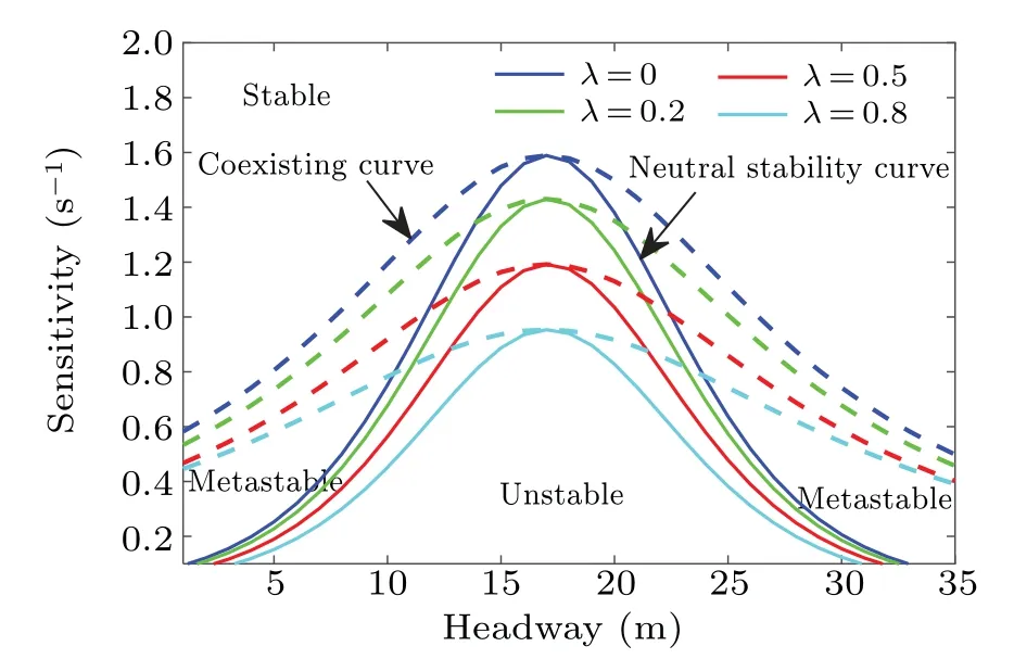
Fig. 2. Phase diagram in the headway-sensitivity space under different λ values.

According to the linear stability condition(22),we check the effect of different model parameters on the stability of traffic flow. The phase diagrams in the headway-sensitivity space under different parametersλandtmare plotted in Figs.2 and 3, respectively. The solid lines represent the neutral stability curves,while the dashed lines denote the coexisting curves.As shown in Figs. 2 and 3, the phase diagram of the traffic flow can be divided into three different areas. Above the coexisting curve is the stable area,below the neutral stability curve is the unstable area, and between the two curves is the metastable area. Figure 2 shows that the self-stabilizing effect in the proposed car-following model can reduce the area of the unstable region, thereby making the traffic flow more stable. In addition, figures 2 and 3 suggest that the unstable area becomes smaller with the increase of the parameterλortm. From these figures,we can draw a conclusion that increasing the value of the parameterλortmcan enhance the stability of the traffic flow and suppress traffic congestion.

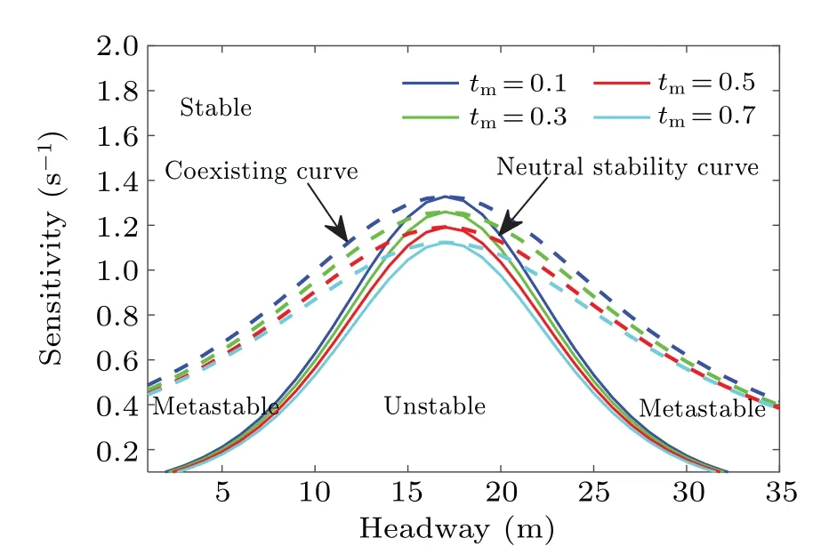
Fig. 3. Phase diagram in the headway-sensitivity space under different tm values.

4. Nonlinear analysis

In this section,the nonlinear analysis is conducted to derive the mKdV equation of the proposed model. First,rewrite the model equation(10)to the following form:

Considering the slow-changing behavior of long waves around the critical point (hc,αc), we define slow variablesXandTas follows:

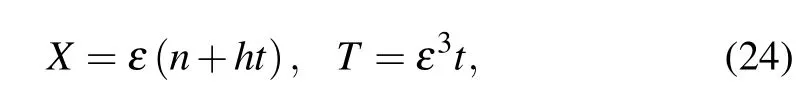
wherenis the space variable,tis the time variable,andhis a constant. The headway can be set as

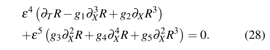
Substituting Eqs. (24) and (25) into the model equation(23)and expanding the equation to termε5yield the following nonlinear partial differential equation:

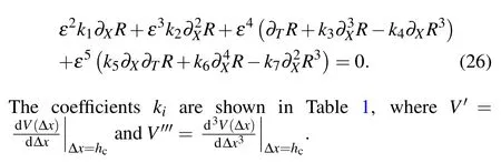
Table 1. The coefficients ki of the model.

If we takeh=V′,then we can eliminate the second-and third-order terms ofε. Near the critical pointτc,let

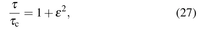
where

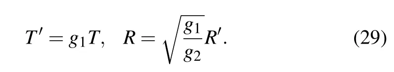
Then equation(26)can be rewritten as follows:

The coefficientsgiare shown in Table 2.

Table 2. The coefficients gi of the model.

The following transformations are conducted to derive the standardized equation:

Then the standard mKdV equation with correction termO(ε)can be deduced:

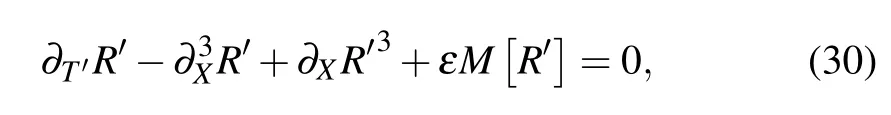
where

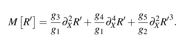
If the correction termO(ε)is neglected,then we can derive the mKdV equation with the following kink–antikink solution:

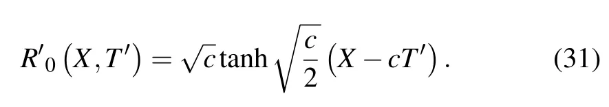
Assume thatR′(X,T′)=R′0(X,T′)+εR′1(X,T′). Here,the correction termO(ε) is taken into consideration. Before determining the propagation velocity value of the kink solution, we need to consider the following solvability condition first:

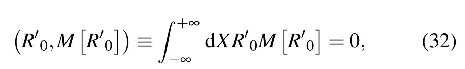
whereM[R′0]=M[R′]. Then the propagation velocity can be calculated,which is expressed by the following formula:

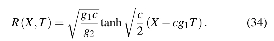
Therefore, the kink–antikink solution of the mKdV equation is given as

The kink–antikink solution of the headway is obtained as follows:

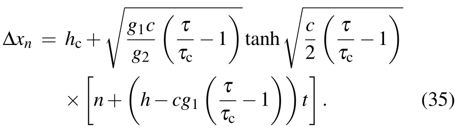
We can also obtain the amplitude of the kink–antikink solution

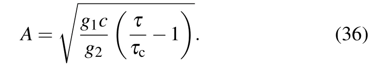
The above kink–antikink solution is used to characterize the coexisting phase of the traffic flow, which includes both the free-running phase and the congested phase. The dashed lines in Figs.2 and 3 depict the coexisting curve of the traffic flow,which can be expressed by Δxn=hc±A.

5. Numerical simulation

To further verify the impact of the self-stabilizing effect on the stability of heterogeneous traffic flow,numerical simulation experiments are carried out in this section.

5.1. Simulation setup

For the convenience of simulation,lett0=mΔt,and then the discrete form of the model(8)can be obtained as

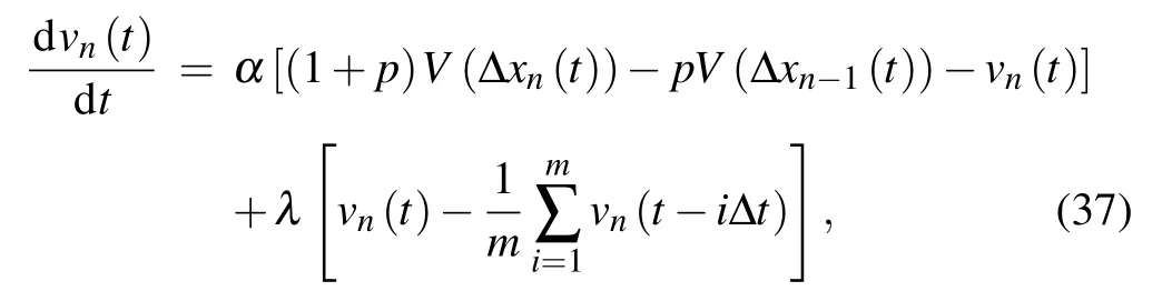
wherep=µfor autonomous vehicles andp=0 for humandriving vehicles[see Eq.(9)].

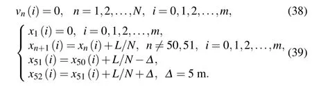
The numerical simulations in this section are conducted under the periodic boundary condition. The road length isL=1700 m and the total number of vehicles isN=100.Without loss of generality, the maximum velocity of all vehiclesisvmax=14.67 m/s and the length of all vehicles is set asln=5 m. The simulation time step is taken as Δt=0.1 s. The simulation duration is 2×105time steps, and the data were picked up at and after the(1.9×105)-th time step.

The initial states of the traffic flow are given as follows:

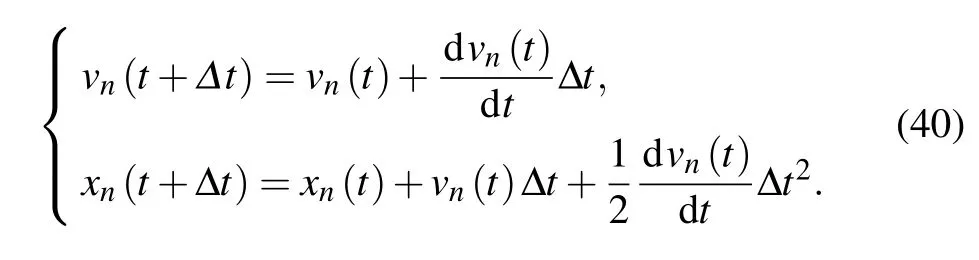
The velocity and position of the vehicles are calculated by the following rules:

5.2. Simulation for autonomous vehicles

In this part,the effect of the self-stabilizing coefficientλand historical time lengtht0on the stability of autonomous vehicle flow is investigated. The model parameters are set as the following values:

(i)αA=1.25,µ=0.1,λ=0,0.2,0.5,0.8,t0=0.5;

(ii)αA=1.25,µ=0.2,λ=0.2,t0=0.1,0.5,1.0,1.5.

The simulation results are shown in Figs.4–7.

Figure 4 shows the headway profiles of autonomous vehicles att=1.9×104s under differentλvalues.From Fig.4,we can see that compared with the model without self-stabilizing effect (λ= 0), the model with self-stabilizing effect has a smaller headway fluctuation, which indicates that the selfstabilizing effect can enhance the stability of autonomous vehicle flow. In addition,with the increase of the self-stabilizing coefficientλ, the headway fluctuation gradually decreases.When the self-stabilizing coefficientλincreases to a certain value, the headway no longer fluctuates. Figure 5 shows the space–time evolution of density waves in autonomous vehicle flow aftert=1.9×104s under differentλvalues. The amplitude of density waves decreases with a greaterλvalue. In addition,the density waves propagate backward with time.

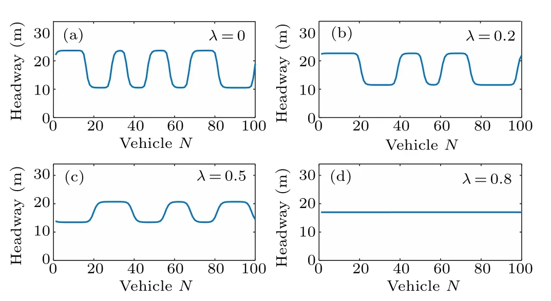
Fig.4. The headway profiles of autonomous vehicles under different λ values at t=1.9×104 s.

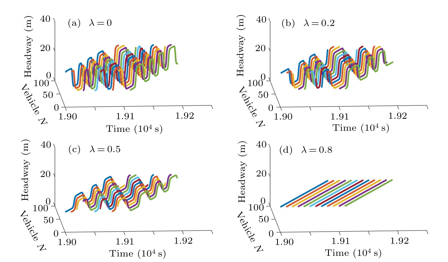
Fig.5. Space–time evolution of density waves in autonomous vehicles under different λ values after t=1.9×104 s.

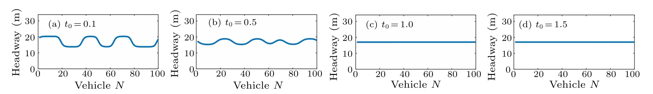
Fig.6. The headway profiles of autonomous vehicles under different t0 values at t=1.9×104 s.

Figure 6 shows the headway profiles of autonomous vehicles att=1.9×104s under different values oft0. As the parametert0increases,the variation range of the headway becomes smaller. Figure 7 shows the space–time evolution of density waves in autonomous vehicle flow aftert=1.9×104s under different values oft0. It can be seen from Fig.7 that increasing the value oft0can decrease the amplitude of density waves.

From the above results,we can conclude that the stability of autonomous vehicle flow is strengthened with the increase of the self-stabilizing coefficient or historical time length. This conclusion is consistent with the theoretical results in Section 3.

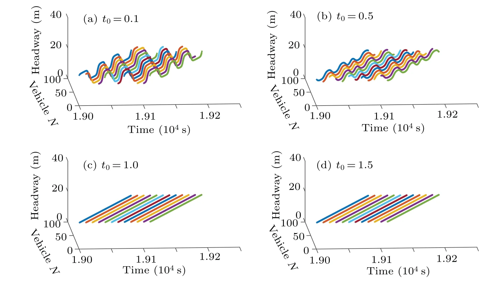
Fig.7. Space–time evolution of density waves in autonomous vehicles under different t0 values after t=1.9×104 s.

5.3. Simulation for heterogeneous traffic flow

In this part,we conduct numerical simulations in heterogeneous traffic flow. First, the influence of different parameters on the stability of heterogeneous traffic flow is studied. In this experiment, human-driving vehicles and autonomous vehicles are 50%respectively,i.e.,the proportion of autonomous vehicles isβ= 0.5. In addition, these two types of vehicles distribute on the road in random order. The sensitivity of human-driving vehicles follows the normal distributionαH～N（0.85,0.052）, and the sensitivity of autonomous vehicles isαA=2.5. The rest of the parameters are taken as follows:

(i)µ=0.2,λ=0,0.2,0.5,0.8,t0=0.5;

(ii)µ=0.2,λ=0.2,t0=0.1,0.5,1.0,1.5.

The results are shown in Figs.8–11.

Figures 8 and 9 show the vehicle trajectories and space–time diagrams of the heterogeneous traffic flow aftert=1.9×104s under differentλvalues,respectively. It can be seen that introducing the self-stabilizing effect in heterogeneous traffic flow can suppress stop-and-go waves and reduce the velocity variation amplitude, so as to enhance the stability of heterogeneous traffic flow. In addition, with the increase ofλ, the stop-and-go waves are gradually dissipated and the velocity fluctuation is gradually reduced.

Figures 10 and 11 show the trajectories and space–time diagrams of heterogeneous traffic flow aftert=1.9×104s under differentt0values,respectively. It is shown that a largert0value means a smaller amplitude of stop-and-go waves and a smaller velocity change.

From Figs.8–11,we can conclude that for heterogeneous traffic flow, increasing the self-stabilizing coefficient or historical time length can also strengthen its stability when the proportion of autonomous vehicles is fixed.

Next, we investigate the relationship between the stability of heterogeneous traffic flow and the proportion of autonomous vehiclesβ. Model parameters are set as:αH～N（0.85,0.052）,αA=2.5,µ=0.2,λ=0.2,t0=0.5, and the proportion of autonomous vehicles are taken asβ= 0,0.33, 0.67, 1. The results are shown in Figs. 12 and 13. As the proportion of autonomous vehicles increases,the stop-andgo waves in the heterogeneous traffic flow are gradually suppressed,and the velocity change is gradually decreased.When the proportion of autonomous vehicles increases to a certain value, the stop-and-go waves disappear in the heterogeneous traffic flow, and the velocity of the heterogeneous traffic flow no longer changes. Therefore, increasing the proportion of autonomous vehicles has a positive effect on stabilizing heterogeneous traffic flow and alleviating traffic congestion.

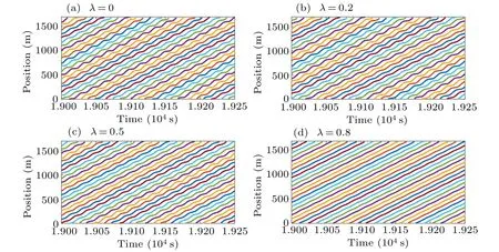
Fig.8. Vehicle trajectories for every five vehicles in the heterogeneous traffic flow after t=1.9×104 s under different λ values(β =0.5).

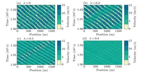
Fig.9. Space–time diagram of heterogeneous traffic flow after t=1.9×104 s under different λ values(β =0.5).

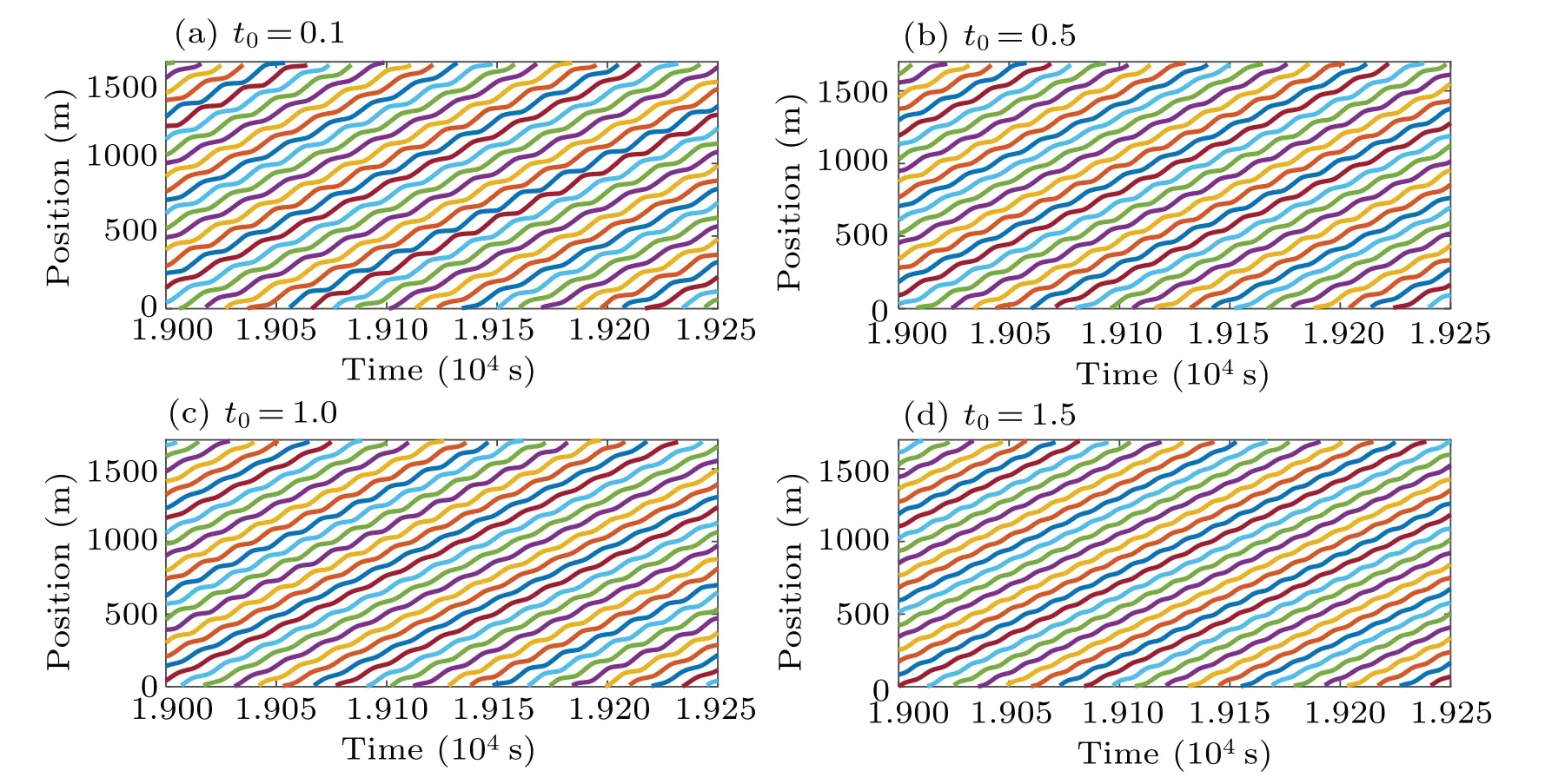
Fig.10. Vehicle trajectories for every five vehicles in the heterogeneous traffic flow after t=1.9×104 s under different t0 values(β =0.5).

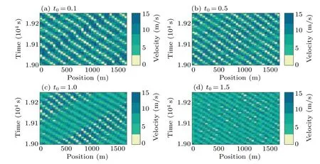
Fig.11. Space–time diagram of heterogeneous traffic flow after t=1.9×104 s under different t0 values(β =0.5).

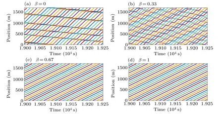
Fig.12. Vehicle trajectories for every five vehicles in the heterogeneous traffic flow under different proportions of autonomous vehicles β after t=1.9×104 s.

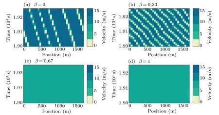
Fig.13. Space–time diagram of heterogeneous traffic flow under different proportions of autonomous vehicles β after t=1.9×104 s.

6. Conclusion and perspectives

In this paper,the heterogeneous traffic flow with humandriving and autonomous vehicles is studied by analytical and numerical methods. First, we propose an extended carfollowing model for autonomous vehicles and heterogeneous traffic flow. It takes into account the self-stabilizing effect of vehicles,which enables the autonomous vehicle to use the information of both its own and other vehicles to jointly control its driving behavior. Through linear stability analysis,we obtain the linear stability criterion of the proposed model. Then,the mKdV equation of the model is derived by nonlinear analysis,and the corresponding kink–antikink solution is obtained.Finally,numerical simulations are performed to verify the analytical results.The results show that the self-stabilizing effect plays an important role in stabilizing the heterogeneous traffic flow. In addition, whether it is homogeneous traffic flow or heterogeneous traffic flow, increasing the self-stabilizing coefficient or historical time length can strengthen the stability of traffic flow and reduce traffic congestion effectively. This conclusion is in good agreement with the theoretical analysis.Moreover, the stability of the heterogeneous traffic flow can also be enhanced by increasing the proportion of autonomous vehicles.

The model proposed in this paper is a theoretical model,and its results mainly come from the simulation data. The future work is to calibrate the model with the data from real traffic so that the model can describe the real traffic behavior more accurately.

Acknowledgements

Project supported by the National Natural Science Foundation of China (Grant No. 61773243), the Major Technology Innovation Project of Shandong Province, China (Grant No.2019TSLH0203),and the National Key Research and Development Program of China(Grant No.2020YFB1600501).