CHEN Yongtang(陈永堂), WANG Qi(王琦)

( School of Mathematics and Statistics, Guangdong University of Technology,Guangzhou 510006, China)

Abstract: This paper is mainly concerned with the numerical stability of delay partial functional differential equations with Neumann boundary conditions.Firstly, the sufficient condition of asymptotic stability of analytic solutions is obtained.Secondly, the linear θ-method is applied to discretize the above mentioned equation, and the stability of the numerical solutions is discussed for different ranges of parameter θ.Compared with the corresponding equation with Dirichlet boundary conditions, our results are more intuitive and easier to verify.Finally, some numerical examples are presented to illustrate our theoretical results.

Key words: Delay partial functional differential equation; Neumann boundary condition;Linear θ-method; Asymptotic stability

1.Introduction

Delay partial functional differential equations (DPFDEs) have been widely applied because of the establishment of models to solve all kinds of problems in nature, science and life[1-5].In spite of this, there are some difficulties in obtaining the analytic solutions[6].So many researchers are constantly looking for precise numerical methods to solve DPFDEs.Among many properties for numerical solutions, stability and convergence are very important,which have aroused wide attention in recent years.Mead and Zubik-kowal[7]investigated delay partial differential equations by a Jacobi waveform relaxation method based on Chebyshev pseudo-spectral discretization, whose convergence speed gradually accelerated when parameteraincreased from 0 to 1.Meanwhile, the error of method decreased with the increase ofaand reached the minimum ata= 1.In [8], an absolutely stable difference scheme with first order accuracy was designed for the study of third-order delayed partial differential equations, while the stability estimate of the three-step difference scheme was obtained.At the same time, the authors continuously researched the existence and uniqueness of bounded solutions for semilinear DPFDEs with the same method.Similarly,ZHAO et al.[9]applied the explicit exponential Runge-Kutta methods to study semilinear DPFDEs.Stiffconvergence and conditional DN-stability of these methods were investigated and the conditions for stiffconvergence order were derived up to fourth order.In [10], Sumit and Kuldeep employed the fitted operator finite difference scheme to discretize the spatial variable and the time variable of the singularly perturbed parabolic differential equations with a time delay and the accuracy in the spatial direction was improved into second order.In addition, Bashier and Patidar[11]designed a robust fitted operator finite difference method for the numerical solution of singularly perturbed parabolic differential equations.This method was unconditionally stable and convergent with orderO(k+h2), wherekandhwere the time and space step-sizes, respectively.Compared with [10-11], Kumar and Kumar[12]used high order parameter-uniform discretization to investigate singularly perturbed parabolic partial differential equations with time delay, which was second order accuracy in time and fourth order accuracy in space.In[13-14], forward and backward Euler scheme and Crank-Nicolson scheme were used to discretize parabolic differential equations with a constant delay, respectively.It was shown that backward Euler scheme and Crank-Nicolson scheme were unconditionally delay-independently asymptotically stable while the forward Euler scheme required an additional restriction on the time and spatial stepsizes.Adam et al.[15]constructed a fitted Galerkin spectral method to solve DPFDEs.They established error estimates for the fully discrete scheme with a Galerkin spectral approximation in space and they found that the numerical solutions were very similar to those obtained by Chebyshev pseudo-spectral method.In [16], a linearized compact difference scheme was presented for a class of nonlinear delay partial differential equations with Dirichlet boundary conditions.The unique solvability, unconditional convergence and stability were discussed.

Different from them, in this study, for the DPFDEs with Neumann boundary condition,we will investigate the stability of numerical solution, which is further extension of [17].By contrast,the stability conditions of linearθ-method in our work are simpler and easier to test,which is the main difference between the two types of boundary conditions.

This paper is organized as follows.In Section 2, a sufficient condition of asymptotic stability of the analytic solutions is given.In Section 3, linearθ-method is used to discretize DPFDEs and the compact form is obtained.Section 4 is devoted to the stability of linearθ-method withθin different intervals.Finally, some numerical experiments are presented to validate the theoretical results in Section 5 and a brief conclusion is given in Section 6.

2.Stability of DPFDEs

In this section, we will give a sufficient condition of asymptotic stability for the analytic solution of the following problem

here parametersr1>0,r2>0, diffusion coefficientsr3∈R,r4∈R, andτ >0 is the delay term.

Definition 2.1The analytic solutionu(x,t)≡0 of Problem (2.1) is called asymptotically stable if its solutionu(x,t) close to a sufficiently differentiable functionu0(x,t) withsatisfies limt→∞u(x,t)=0.

Theorem 2.1Assume that the solution of Problem (2.1) isu(x,t) = eλtcos(nx),whereλ ∈C,n ∈N+,x ∈[0,π] andt >0.Then the analytic solution of Problem (2.1) is asymptotically stable for

and unstable for

ProofLetX=B[0,π]be the Banach space equipped with the maximum norm.DefineD(A)={y ∈X:∈X,0)=(π)=0}andAy=fory ∈D(A).

Let−r1n2(n= 1,2,···) be the eigenvalues ofA.According to Theorem 3 in [17], if all zeros of the following characteristic equations

have negative real part,then the analytic solution is asymptotically stable.At the same time,if at least one zero has positive real part, then it is unstable.

Denoteλ=u+vi,u,v ∈R.Letf(λ)=0, thenu+vi=r3−r1n2+(r4−r2n2)e−uτ−vτi.Separating the real and imaginary parts, we arrive at

Now, assume the real partu <0, thenr3−r1n2< −(r4−r2n2)e−uτcosvτ.Due tov=−(r4−r2n2)e−uτsinvτhave some roots in R, then−(r4−r2n2)>0.So we haver3−r1n2<−(r4−r2n2)e−uτcosvτ ≤−(r4−r2n2).

If(2.2)holds,then all zeros of the characteristic equations have negative real part.Therefore, the analytic solution of Problem (2.1) is asymptotically stable.

If (2.3) holds, then there exists a zeroλ0with positive real part such thatf(λ0) = 0,which implies the analytic solution is unstable.

Thus, the proof is completed.

3.Linear θ-Method

Let Δx= π/N,N ∈N+be the space step size and Δt= 1/m,m ∈N+be the time step size, respectively.Denotexj=jΔx(j= 0,1,2,··· ,N),tk=kΔt(k= 0,1,2,···), thenxjandtkconstitute a uniform space-time grid diagram.Letbe the numerical approximation ofu(xj,tk) and the linearθ-method of Problem (2.1) can be defined as:

From the first part of (3.1), we have

where

Thus, (3.1) can be written as:

where

4.Asymptotic Stability of Linear θ-Method

In this section, we will discuss the asymptotic stability of the numerical solution of Problem (2.1).

Definition 4.1A numerical method applied to Section 3 of Problem (2.1) is called asymptotically stable ifclose to a sufficiently differentiable functionu0(x,t)with=0 satisfies

According to Section 3 of [17], if we want to verify the numerical solution being asymptotically stable, we need to prove that

is a Schur polynomial for anym ≥1, whereλjis thej-th eigenvalue of the matrixSandλj=2 cos(jΔx),j=0,1,2,··· ,N.[18]

Therefore, it is necessary to introduce a corresponding lemma that we can prove (4.2) is a Schur polynomial .

Lemma 4.1[17]Letγm(z) =α(z)zm −β(z) be a polynomial, whereα(z) andβ(z) are polynomials of constant degree.Thenγm(z) is a Schur polynomial for anym ≥1 if and only if the following conditions hold

(i)α(z)=0⇒|z|<1;

(ii)|β(z)|≤|α(z)|,∀z ∈C,|z|=1;

(iii)γm(z)0,∀z ∈C,|z|=1,∀m ≥1.

Denote

then

Theorem 4.1Under the condition(2.2),suppose that 4e1>e3,4e2>e4, e3<0,e4<0 and−e3>4e2−e4.Then (3.1) is asymptotically stable forθ ∈[0if and only if

whereei(i=1,2,3,4) are defined in (3.2).

Proof(Necessity) First of all, we prove the item (i) of Lemma 4.1.Fromφj(z)=0 we can derive

In order to verify|βj(z)| ≤|αj(z)|,∀z ∈C, |z|= 1, j= 0,1,2,··· ,N, we set up a function defined in complex domain

Lettingw=x+yi, after some basic simplifications, we obtain

In a word, whereas after (a) and (b) have been discussed, we conclude that, for allz ∈C,|z|=1,φj(z)>ψj(z),j=0,1,2,··· ,Nholds.At this point, the items (ii) and (iii) of Lemma 4.1 have been proved.

By the above analysis, we conclude that (3.1) is asymptotically stable with the help of Lemma 4.1.

(Sufficiency) We prove in two opposite ways:

(a) If (4e1+4e2−e3−e4)(1−2θ)=2, we takemto be odd,j=Nandz=−1.Then for|z|=1, we observe that1)=0, which is in conflict with condition (iii) of Lemma 4.1.Thus, (3.1) is not asymptotically stable.

(b) Assume that (4e1+4e2−e3−e4)(1−2θ)>2.Letmbe odd,j=Nandz=−1,then we get|ψj(−1)| > |φj(−1)|.This confirms that condition (ii) of Lemma 4.1 does not hold, so (3.1) is not asymptotically stable.

Therefore, (4.5) is a necessary condition for asymptotic stability.This proof is finished.

Next, we will prove that (3.1) is unconditionally asymptotically stable forθ ∈

Theorem 4.2Under the condition(2.2),suppose that 4e1>e3,4e2>e4,e3<0,e4<0 and−e3>4e2−e4.Then (3.1) is unconditionally asymptotically stable for

ProofFirst of all, due toφj(z)=0, we arrive at

which is similar to the proof of Theorem 4.1.

Then, in order to verify the items (ii) and (iii) of Lemma 4.1, we define the following function

(a)θ=Setw=x+yi and|z|=1.After some reductions, we get

By the conditions 4e1> e3,4e2> e4,e3<0,e4<0,−e3>4e2−e4and 4e1−e3≥e1(2−λj)−e3≥−e3>4e2−e4≥e2(2−λj)−e4≥−e4>0, we find that

which confirms the items (ii) and (iii) of Lemma 4.1.

(b)].In the same way, we arrive at

In this case, for allz ∈C,|z|=1, we also obtain that

This completes the proof.

5.Numerical Experiments

In this section, some numerical experiments are carried out to illustrate the theoretical results.Consider the following problem:

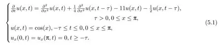
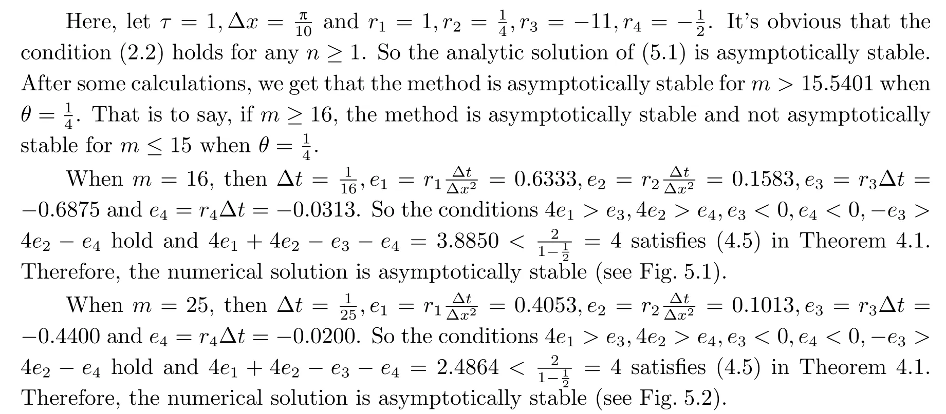
Fig.5.1 The numerical solutions of Problem (5.1) with m=16 and θ =

Fig.5.2 The numerical solutions of Problem(5.1) with m=25 and θ =

Fig.5.3 The numerical solutions of Problem (5.1) with m=30 and θ =

Fig.5.4 The numerical solutions of Problem(5.1) with m=14 and θ =

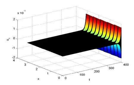
Fig.5.5 The numerical solutions of Problem (5.1) with m=15 and θ =

Fig.5.6 The numerical solutions of Problem(5.1) with m=5 and θ =0.5

Fig.5.7 The numerical solutions of Problem (5.1) with m=8 and θ =0.6

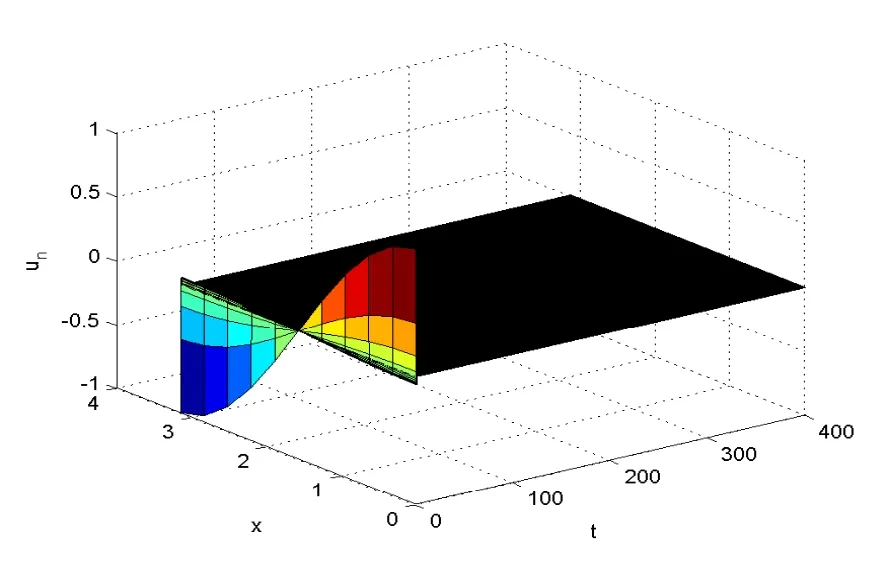
Fig.5.8 The numerical solutions of Problem(5.1) with m=15 and θ =0.6

Fig.5.9 The numerical solutions of Problem (5.1) with m=25 and θ =0.8

Fig.5.10 The numerical solutions of Problem(5.1) with m=50 and θ =0.8

6.Conclusion

The linearθ-method for solving DPFDEs with Neumann boundary conditions is proposed in this paper.The asymptotic stability condition of the analytic solutions and the numerical solutions are derived, respectively.Compared with DPFDEs with Dirichlet boundary conditions[17], it is shown that the stability condition is more intuitive and effective.In our future work, we will consider the multidimensional problem.