Yang Li Ma Yinhang Jin Juan Yang Fujun Yang Fang Huang Bin Li Yan Gu Ning

(1School of Biological Science and Medical Engineering, Southeast University, Nanjing 210096, China)(2State Key Laboratory of Bioelectronics, Southeast University, Nanjing 210096, China)(3Jiangsu Key Laboratory for Biomaterials and Devices, Southeast University, Nanjing 210096, China)(4 School of Civil Engineering, Southeast University, Nanjing 210096, China)

Abstract：A novel method combining visualization particle tracking with image-based dynamic light scattering was developed to achieve the in situ and real-time size measurement of nanobubbles (NBs). First, the in situ size distribution of NBs was visualized by dark-field microscopy. Then, real-time size during the preparation was measured using image-based dynamic light scattering, and the longitudinal size distribution of NBs in the sample cell was obtained in a steady state. Results show that this strategy can provide a detailed and accurate size of bubbles in the whole sample compared with the commercial ZetaSizer Nano equipment. Therefore, the developed method is a real-time and simple technology with excellent accuracy, providing new insights into the accurate measurement of the size distribution of NBs or nanoparticles in solution.

Key words：real-time acquisition; nanobubble (NB) sizing; visualization particle tracking; image dynamic light scattering; Brownian motion

In the past two decades, nanobubbles (NBs) have attracted increasing attention from researchers in biology, medicine, and the environment[1-2]. NBs with a size range of 10-3to 100μm are fabricated with innovative technologies[3-5]. In biomedical applications, NBs can extravasate from the vascular lumen, and their accumulation at target sites can be mediated via the enhanced permeability and retention (EPR) effect[6]. Thus, determining the accurate size of NBs is important, especially in biomedical applications.

Several techniques have been used to measure the hydrodynamic size of bubbles, and the image method, laser-diffraction particle-size analyzer[7-8], and dynamic light-scattering (DLS) method[9-10]are the most typical. The shrinking of macro-bubbles to microbubbles can be recorded with a high-speed camera attached to an inverted microscope[11]. Nevertheless, measuring the size during NB generation remains challenging because the size varies very fast as large bubbles shrink to NBs[12]. A laser-diffraction particle-size analyzer based on the light-scattering properties of bubbles can be used to measure sizes ranging from approximately 0.1 μm to 3 mm. Based on the Brownian motion of particles, DLS method is also used to measure the size and size distribution of nanoparticles in solution or colloidal suspensions. In the conventional DLS method, the scattered light by nanoparticles is received by a photon multiplier tube or avalanche photodiode. Then, the measured one-point scattered signals are processed by digital correlators to obtain the time-intensity autocorrelation functions (ACFs). Given the randomness of the Brownian motion, the ACFs should be averaged among different time-series data to obtain a reliable and stable result. Therefore, one measurement can take tens of seconds to more than hundreds of seconds. This process cannot acquire the first-time size of bubbles during NB preparation. In situ size measurements are very helpful in the preparation of nanoparticles or NBs and in studies on formation mechanisms. Obviously, existing methods are unsuitable for in situ size measurements of nanoparticles and NBs. Thus, a new method to achieve in situ and in real-time size measurements of nanoparticles and NBs needs to be developed.

Dark-field microscopy (DFM) is a powerful tool to directly image the scattered light generated from nonhomogeneous materials. The diameter of single gold nanoparticles could be estimated by using the chrominance of scattering light captured by DFM[13]. The trajectories of single oxygen nanobubble can be tracked with DFM[14]. Our previous research has proven that DFM is also an effective means to track bulk NBs dynamically[15]. The evolution of single bubbles from micro to nano size has been monitored with continuous DFM imaging. The individual NB motion in bulk water has also been tracked with DFM, but the size distribution of nanobubbles remains to be determined.

With the rapid development of image sensors in recent years, using a charge-coupled device (CCD) or complementary metal-oxide-semiconductor (CMOS) camera as an area detector to replace the conventional detector is a promising way to decrease the measuring time in DLS measurement. Xu et al.[16]and Zhou et al.[17]proposed the fast sizing method (imaged-based DLS) to size mono-dispersed standard latex particles in water under high-speed camera capture. This approach can shorten the acquisition time to milliseconds by setting the frame rate of CCD from thousands of frames per second. In our opinion, imaged-based DLS (IDLS) may realize the in situ size measurements of nanoparticles and NBs.

In the present study, the motions of almost all NBs in the field of DFM were tracked visually. Then, the trajectories of NBs were analyzed to estimate the size distributions of NBs in bulk water. Moreover, IDLS was employed to measure the diameter in real time during NB preparation for the first time. In this method, the size of the bubbles at five time points during the preparation was obtained using IDLS integrated with the reformulated versions of the cumulant method[18-19]. The average size of the bubbles decreased from 1 202.4 to 237.7 nm within about 1 min, demonstrating the dynamic size change from micro to nano after preparation. Then, in the steady state, the longitudinal size distribution of the NBs was further measured at three positions in the longitudinal direction. The bubbles in the upper and middle position were larger than those in the bottom position. This result was verified with IDLS. Thus, compared with the previous method, the proposed method can obtain a more accurate and detailed size distribution of NBs.

1 Experimental Section

1.1 Materials

Ultrapure water with a resistivity of 18.25 MΩ·cm was prepared with a purification system (Youpu Ultrapure Technology Co., Ltd., China). The ultrapure water was used to generate NBs and to dilute the samples. SF6with a purity of 99.99% was purchased from Anhui Qiangyuan Gas Co., Ltd. (Wuhu, China).

1.2 Preparation of the NBs

SF6gas bubbles were fabricated in accordance with the repeated compression method reported in the literature[15,20]. In brief, a 3 mL bottle was filled with 2 mL of ultrapure water, and the medical syringe was filled with 3 mL of SF6gas. The syringe and the bottle formed an airtight system. The syringe piston can move up and down in the vertical direction so the gas can be pushed into the bottle and pumped back into the syringe. Owing to the sealed system, the pressure inside the bottle changed as the syringe inhales and expels the SF6gas. NBs were prepared by pushing and pumping repeatedly (about 100 to 200 times) and then leaving the sample cell for a period of time.

1.3 Measurement with dark-field microscopy

The freshly prepared and diluted NBs were taken out and dropped on the clean glass slide. Dark-field measurements were performed on an inverted microscope (Nikon Ti2-U, Japan) equipped with a dark-field condenser (0.95 to 0.80). The white collimated LED lamp source (TI2-D-LHLED, Japan) focused through the dark-field condenser was used to illuminate the NB dispersion (see Fig.1). The scattering light of NBs was collected by a 40× objective and detected by an CCD camera with frame rate of 30 frames/s. Image data were collected as a 30 s movie using NIS-Elements D software. All samples were observed by DFM at room temperature and atmospheric conditions.

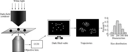
Fig.1 Schematic of visualization size measurement of nanobubbles based on DFM

1.4 Visualization particle trajectory and size distribution calculation

The motions of NBs were recorded as a movie through DFM imaging. The single-particle tracking method[15]was used to locate the spatial positions of these bright individual NBs over time. TheXandYcoordinates of the bright spots were obtained for all frames of the movie. Thus, data sets consisting of an NB’s 2D trajectory were extracted. For each NB, the mean-square displacement (MSD) can be calculated for every time interval (1/30 s). The diffusion constants of NBs can be obtained on the basis of the MSD[21]. Our previous study[15]has proven the Brownian motion of NBs. Thus, the diameter of NBs can be calculated from the Stokes-Einstein equation as follows:

(1)

wheredis the diameter of NBs;kBis the Boltzmann constant;Tis the absolute temperature;ηis the viscosity of the fluid; andDis the diffusion constant of NBs. All diameters of bright spots in the image can be calculated to obtain the size distribution of NBs (see Fig.1). The average diameter can be obtained by repeating this process three times.

1.5 IDLS apparatus and calculation method

The bubble preparation device and IDLS measurement system are shown in Fig.2. The vial bottle (clear glass) was used for bubble preparation and size measurement. A green solid-state laser system at 532 nm with 20 mW was used as a light source. The laser beam was focused by a lens with focal lengthf= 60 mm inside the sample cell. The focal spot was positioned in the center of the bottle with an inner diameter of 14 mm and a height of 35 mm. An adjustable diaphragm was applied to define the measured scattering area with an opening diameter of 0.5 mm in the experiment. The limited light signal was captured as images by a CMOS camera (FASTCAM SA3) at a scattering angleθ=45° (this angle was chosen to balance the density of scattered light and speckle dynamics).

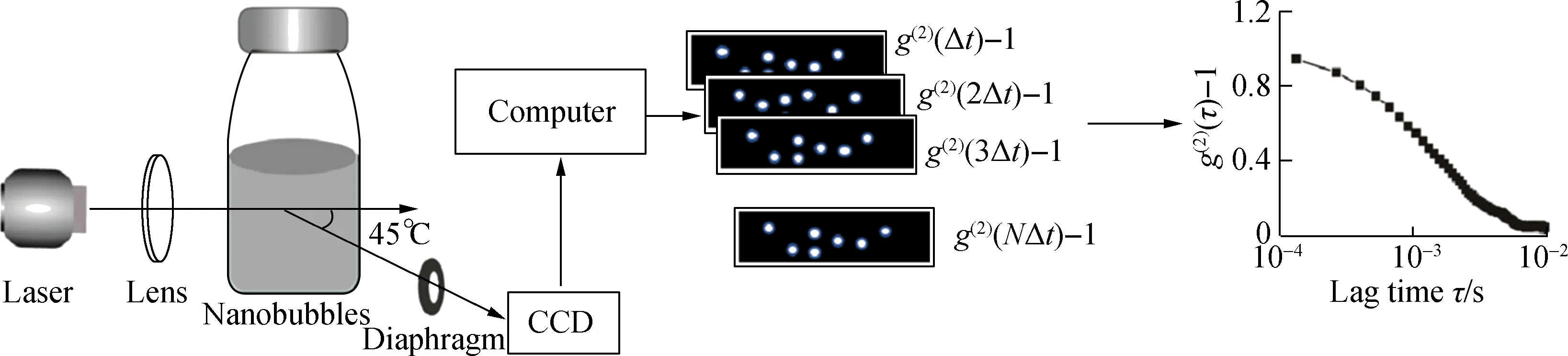
Fig.2 Schematic of IDLS measurement device

The detailed description about DLS theory can be found in previously published papers[18,22-23]. Here the reformulated versions of the cumulant method and cross-correlation analysis are illustrated briefly as follows.

The normalized field correlation functiong(1)(τ) can be expanded in terms of the cumulants of the distribution, andg(2)(τ) can be fitted with the nonlinear least-square method as

(2)

The ACFs can be fitted using cross-correlation analysis[17]between two images. A time series of images was captured using a camera with a constant frame rate. The images are in the same time intervals. The calculation method of the ACF from a time series of images with the same time intervals is shown in Fig.2. The cross-correlation processing between the first and second images determined the first value of the ACF with a lag time, whereas that between the first and third images decided the second value of the ACF with two times lag. The first and the last one determined the last value of the ACF.

1.6 Diameter measurement with IDLS

The longitudinal size distribution of NBs in the bottle was measured using IDLS. The coherence area and frame rate of the camera were the same as above, the camera resolution was selected as 400×110 pixels, and the frame rate of the camera was set as 7 500 frames per second in this part. The liquid level was about 1.4 cm high. From the bottom up, the bubble sizes at 0.3, 0.7, and 1.1 cm were measured.

2 Results and Discussion

2.1 Size distribution calculation by visualization particle tracking

The scattering light of the NBs was recorded as bright spots in the DFM image shown in Fig.3(a). Each NB is represented by a spot, and the brightness of the spot indicates its size. Trajectories of 2D displacement for NBs in aqueous solution were recorded in DFM movie for 30 s. The frame rate of the movie was 30 frame/s. The NBs that moved out of sight were eliminated. The motions of 24 NBs are depicted as curves with different colors. Each curve contains 900 points and represents the trajectory of one NB (see Fig.3(a)). The irregular curves suggest the irregular random motion of the NBs in aqueous solution. Subsequently, we used the single-particle tracking method to locate the spatial positions of these bright individual NBs over time. TheXandYcoordinates of each NB can be obtained for all frames of the movie. Trajectories of three randomly selected NBs (circled as No. 1, No. 2, and No. 3) during 3 s are shown in Figs. 3(b) to (d). The displacement distributions along theXandYcoordinates of the three NBs are shown by histogram in Figs. 4(a) to (f), and the black dotted lines show Gaussian fits. These irregular random motions and Gaussian displacement distributions indicate the Brownian motion of the NBs in bulk water.

The MSDs of the three NBs were calculated during a time interval of 0.03 s and are presented in Fig.5(a). The MSD vs. time is approximately linear, and the corresponding diffusion constants were estimated from the slope of the plots. The diffusion constants for No. 1 to No. 3 NBs are 2.5, 1.7, and 1.2 μm2/s, respectively. The diameter of the NBs can be calculated based on the Stokes-Einstein relationship. The corresponding diameters are 175.7, 260.3, and 369.6 nm, respectively. The diffusion constants and particle diameter have an inverse relationship.

On the basis of the trajectories of the 24 NBs, all the MSDs of these NBs were calculated and are shown in Fig.5(b). The corresponding diameter can be worked out. The statistical size distribution of the NBs in DFM movie was obtained using the frequency statistics method. Each test was repeated for three times. As shown in Fig.5(c), the distributions indicate that the estimated diameters of NBs are approximately (322.6 ±24.1) nm and the dotted line shows Gaussian fit. The size distribution result was verified with a commercial Zetasizer Nano equipment (Nano ZS90, Malvern Instrument, United Kingdom).Fig.5(d) shows the NBs’ size distributions obtained by calculating the scattering light intensity. The distributions indicate that the estimated diameters of the NBs are approximately (264.3 ±5.2) nm. The average difference between the calculated diameters by visualization particle tracking, and the DLS is approximately 60 nm. The reason could be that the bright spots were more easily observed. Furthermore, the big NBs floated upward because of buoyancy.

2.2 Diameter measurement during bubbles preparation

The pushing and pumping processes were repeated about 200 times. After the gas and water in the syringe were pressed into the bottle, the needle was pulled out. At the beginning, large and small bubbles appeared in the bottle, and then the large bubbles shrank into small ones quickly. After approximately 10 to 20 min, only NBs were left in the bottle. The Tyndall phenomenon was used to confirm this process, which is shown in Fig.6. The Tyndall phenomenon did not occur when a laser beam irradiated the ultrapure water while a light path was present in the aqueous bubble solutions. As shown in Fig.6(a), the Tyndall scattered signals were unhomogeneous and strong in the aqueous bubble solutions immediately after the NB preparation. After storage for 10 min, a thinner and homogeneous light path appeared in the NB solutions, as shown in Fig.6(b).

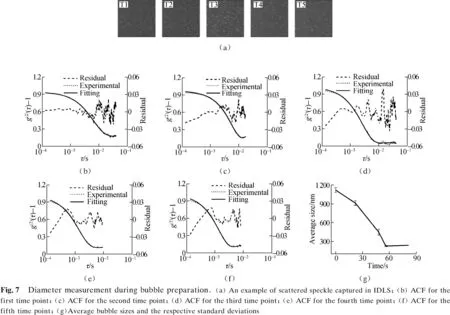
The size measurement during the bubble preparation was based on IDLS. The bubble size changes at five time points (0, 22, 48, 56, and 80 s) during the preparation were measured. The frame rate of the camera was set as 6 000 frames per second. Then, 300 couples of images were captured continuously at each time step. Each test was repeated three times. Examples of scattered speckle (enhanced for display) captured in IDLS are shown in Fig.7(a). Figs.7(b) to (f) display the fit (solid line) to experiment data (dotted line) of ACF. Residuals (dash line) or the difference between experiment data and fit is also indicated. The small residuals indicate the good fit between the experiment and calculation data. The time to the minimum values of ACF ranges from 22.7 to 5.2 ms, which means the size of the bubbles varied from large to small. The average hydrodynamic diameters of the bubbles can be obtained and are shown in Fig.7(g). The average bubble size and the respective standard deviations for each test, together with the values ofPDIcalculated from Eq.(2), are listed in Tab.1. The bubble size varied from 1 202.4 nm to 237.7 nm before finally stabilizing at about 230 nm. The microbubbles take about 56 s before shrinking to NBs. This period is much longer than the bubble shrinkage time reported in Ref.[12]. The reason may be that the oversaturate solution slows down the shrinking rate of the bubbles. Furthermore, the NBs formed at different times in the vial bottle. This phenomenon also caused the wide particle-size distribution of the bubbles during the preparation.

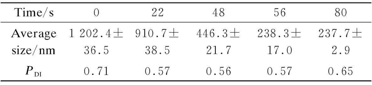
Tab.1 Measurement results for NBs by IDLS

2.3 Longitudinal size distribution measurement for NBs

The longitudinal diameter distributions of the NBs (prepared after 15 min) were measured with the apparatus shown in Fig.2. We define the three positions of the sample cell (the liquid level in the sample cell was 1.4 cm) at 0.3, 0.7, and 1.1 cm as bottom, middle, and upper, respectively. Examples of scattered speckle captured by IDLS for the NBs are shown in Fig.8(a). The images were enhanced for display. Figs. 8(b) to (d) show the fit (solid line) to experiment data (dotted line) of ACF. Residuals (dash line) or the difference between experiment data and fit is also indicated. The small residuals indicate the good fit between the experiment and calculation data. The longitudinal diameter distributions of NBs can be obtained and the average sizes of the NBs at the upper, middle, and bottom positions are 340.3, 347.6, and 228.4 nm, respectively. This result indicates that the NBs are stratified vertically because the density is less than that of water. The average sizes of the NBs at the upper and middle positions agree well with the results measured by visualization particle tracking. A summary of the measurement results of the average size of the NBs andPDIis shown in Tab.2.

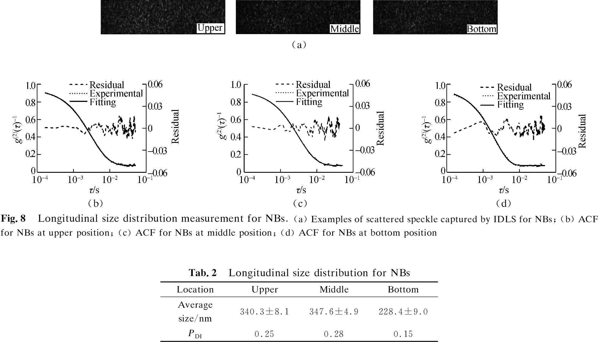
(a)(b) (c) (d)Fig.8 Longitudinal size distribution measurement for NBs. (a) Examples of scattered speckle captured by IDLS for NBs; (b) ACF for NBs at upper position; (c) ACF for NBs at middle position; (d) ACF for NBs at bottom positionTab.2 Longitudinal size distribution for NBsLocationUpperMiddleBottomAverage size/nm340.3±8.1347.6±4.9228.4±9.0PDI0.250.280.15

Furthermore, the size measurement of the NBs was verified with a commercial Zetasizer Nano equipment (Nano ZS90, Malvern Instrument, United Kingdom). A 1 mL solution of NBs was removed in the sample cell when they reached a steady state and were measured by Nano ZS90. The obtained values of the mean size are the arithmetically calculated values for a triplicate experiment. The average size of NBs is 230.9 nm, which agrees well with size measured with IDLS.

3 Conclusions

1) A method combining visualization particle tracking with DFM was developed to estimate the size distributions of NBs. The NB size could be visually quantified in situ.

2) IDLS was used to in situ measure the average size of the bubbles and dynamically monitor the size change during bubble preparation. After preparation, the average size of the bubbles gradually decreases from 1 202.4 nm to 237.7 nm and finally stabilizes at about 230 nm. The NB size remains steady and then becomes stratified by size in the sample cell. This phenomenon is confirmed by measuring the longitudinal size distribution. The average size of the NBs in one position is also verified by a commercial Zetasizer Nano equipment.

3) The proposed method can be used to size polydisperse particles or bubbles in situ, especially when the particle size needs to be accurately determined.