Sheng Fang ,Yanding Wei,,Lei Fu ,Geng Tian ,Haibin Qu

1 The State Key Laboratory of Fluid Power and Mechatronic Systems,College of Mechanical Engineering,Zhejiang University,Hangzhou 310027,China

2 Key Laboratory of Advanced Manufacturing Technology of Zhejiang Province,College of Mechanical Engineering,Zhejiang University,Hangzhou 310027,China

3 College of Mechanical Engineering,Zhejiang University of Technology,Hangzhou 310023,China

4 Pharmaceutical Informatics Institute,College of Pharmaceutical Sciences,Zhejiang University,Hangzhou 310058,China

Keywords:Conical fluidized bed Negative pressure Pressure fluctuation Time-series analysis Characteristic value Fluidized state

ABSTRACT The negative pressure conical fluidized bed is widely used in the pharmaceutical industry.In this study,experiments based on the negative pressure conical fluidized bed are carried out by changing the material mass and particle size.The pressure fluctuation signals are analyzed by the time and the frequency domain methods.A method for absolutely characterizing the degree of the energy concentration at the main frequency is proposed,where the calculation is to divide the original power spectrum by the average signal power.A phenomenon where the gas velocity curve temporarily stops growing is observed when the material mass is light,and the particle size is small.The standard deviation and kurtosis both rapidly change at the minimum fluidization velocity and thus can be used to determine the flow regime,and the variation rule of the kurtosis is independent of both the material mass and particle size.In the initial fluidization stage,the dominant pressure signal comes from the material movement;with the increase in the gas velocity,the power of a 2.5 Hz signal continues to increase.A method of dividing the main frequency by the average cycle frequency can conveniently determine the fluidized state,and a novel concept called stable fluidized zone proposed in this paper can be obtained.Controlling the gas velocity within the stable fluidized zone ensures that the fluidized bed consistently remains in a stable fluidized state.

1.Introduction

As highly efficient material exchange equipment,fluidized beds are widely used in various industries such as combustion,separation,water treatment.In the pharmaceutical field,fluidized beds can be used in granulation [1],drying [2],and coating processes[3].Moreover,the pharmaceutical fluidized bed has become increasingly popular,mostly because multiple processes can be carried out using the same equipment,which greatly improves productivity and makes it easier to achieve a completely sterile environment.Through the investigation of many kinds of pharmaceutical fluidized beds,it is found that the conical fluidized beds are more widely used than cylindrical fluidized beds [4].Since the conical fluidized bed has a gas velocity gradient[5]in the axial direction,that is,the average gas velocity of the upper layer is smaller than that of the lower layer,the coarse particles of the lower layer can be well fluidized,and the entrainment of the fine particles in the upper layer can be weakened.This property makes the conical fluidized bed particularly suitable for the fluidization needs of materials with a wide particle size distribution and for the maintenance of a stable fluidized state over a wide range of gas velocities[6].In addition,a significant difference between most pharmaceutical fluidized beds and other fluidized beds is that the gas-driven equipment(usually a high-pressure fan)is placed at the outlet of the gas path.This design makes the entire interior of the equipment(the fluidization chamber and ventilation duct)a negative pressure environment;thus,this type of fluidized bed is also called a negative pressure fluidized bed.The reason for this design is that a negative pressure vessel is safer than a positive pressure vessel if there is leakage,and the material does not scatter everywhere,which would cause contamination.Besides,the internal negative pressure environment makes it convenient to add materials during operation,because the materials can be inhaled into the fluidization chamber by the pressure difference.Moreover,in the negative pressure fluidized bed,the gas passes through the fluidization chamber from the bottom to the top,and then enters the fan through a long downward pipe.Therefore,the gas channel between the fan and the fluidization chamber is relatively long compared with the design of setting the fan at the inlet (positive pressure bed),which makes the gas flow more uniform and avoids the high-frequency vibration at the fan from affecting the fluidization quality.

The pressure fluctuation signal in a fluidized bed is a very common and important signal,which is very reliable,easy to measure and can be used in sterile,high temperature and high humidity environments.The accuracy and response speed of the pressure sensor are generally at fairly high levels,and the price is also relatively inexpensive.In a negative pressure fluidized bed,there are still pressure fluctuations and pressure drops similar to those of a positive pressure fluidized bed.Pharmaceutical fluidized beds used in practice often have pressure measuring ports in some key sites,such as the plenum or the front and back of the filter bag,for monitoring the current fluidized state.However,the current detection methods are relatively simple.For example,if it is observed that the negative pressure in the plenum is too large,the air inlet may be blocked.If the pressure drop between the front and back of the filter bag is too large,it tells that the dust accumulation in the filter bag may be serious,and it is necessary to perform the dust removal vibration operation or wash the filter bag.The pressure fluctuations are related to many factors.L.T.Fan et al.[7] noted that the pressure fluctuations in the upper layer were mainly caused by bubble movement,and in the lower layer,they were caused by a combination effect from the formation of large bubbles in the middle portion,the formation of small bubbles near the distributor,and the jet flow above the distributor.Hsiaotao T.Bi[8]believed that the local pressure fluctuations came from local bubble-induced fluctuations,global bed oscillations and pressure waves that originated in other locations.J.van der Schaaf et al.[9]suggested that the measured pressure fluctuations were due to the combination effect of fast and slow pressure waves.The fast pressure waves included the upward pressure waves originating from bubble formation and bubble coalescence,and the downward pressure waves caused by bubble eruption at the surface.The slow pressure waves only moved upward and came from rising bubbles.

There are many factors that affect the flow behavior of the fluidized bed,among which the particle size and material mass are the most basic and influential factors.In the process of granulation or coating in the fluidized bed,the particle size and material mass will change in real-time,so monitoring the real-time value of these two factors is the subject studied by many scholars,so this paper chooses to explore these two factors in detail.Along with the development of time-series signal processing technology,many mathematical methods have been applied to analyze the pressure fluctuation time-series signals,which include the time domain analysis [10–12],frequency domain analysis [13–15],and chaotic analysis[16–18].Some studies[19–26]have made use of multiple methods and generally obtained more accurate and complex conclusions.The scholars of these studies have found that the pressure fluctuation signals contain much more information,which can be used to monitor particle size/moisture content/bubble size[10,23],monitor and control flow regimes and their transitions[11,15,19,21,24–26],detect and provide early warning of the defluidization phenomena [13,17,21,26],analyze the hydrodynamic characteristics during drying process [14,16],etc.

Since the FDA (Food and Drug Administration) proposed the process analytical technology (PAT) requirements,many scholars have proposed various methods to monitor the fluidized state in pharmaceutical fluidized beds.T.Pugsley et al.[27]proposed many methods to monitor the drying process,such as electrical capacitance tomography(ECT),high-frequency pressure fluctuation analysis and radioactive particle tracking (RPT).Lilian de Martín et al.[23] compared three pressure fluctuation analysis methods used to monitor the drying and granulation processes.Anneleen Burggraeva et al.[28] reviewed various process analytical techniques in fluidized bed granulation.Carlos Alexandre M.da Silva et al.[29] reviewed the monitoring and control techniques of the fluidized state,particle size and moisture content during the coating and granulation processes.

However,until now,no scholar has systematically studied the pressure fluctuations of the negative pressure conical pharmaceutical fluidized bed;most of the research objects in published studies are positive pressure cylindrical fluidized beds,and the conclusions drawn based on the latter cannot be directly applied to the former.In this study,we focused on two influencing factors that affect the flow behavior of fluidized beds:material mass and particle size.By changing the values of the two influencing factors,several experiments were carried out,and the pressure fluctuation signals were recorded at different gas velocities.The measured pressure fluctuation time-series signals were analyzed using many mathematical methods in an attempt to find the correspondence between the characteristic values obtained by these methods and the influencing factors or the fluidized state.On the one hand,this approach can be used as an auxiliary monitoring method for the two influencing factors in actual production.On the other hand,this approach can also help operators more accurately analyze the current fluidized state.

2.Experimental

2.1.Experimental equipment

The experimental equipment was an experimental pharmaceutical granulation/drying fluidized bed(FBL-10,Xiaolun Pharmaceutical Machinery,China).The tapered portion was detachable and is referred to as the conical cylinder in this paper.The diameter of the bottom and top of the conical cylinder were 180 mm and 300 mm,respectively,the height was 384 mm and the tapered angle was 17.76°.As shown in Fig.1,at the bottom of the conical cylinder was a gas distribution plate used for supporting materials and ventilation,which was made of stainless steel and had a thickness of 3 mm.There were many holes arranged in a square array mode on the gas distribution plate.The diameter of each hole was 1.6 mm,and the interval between two holes was 4 mm,so the overall opening ratio was calculated to be 12.78% by counting the number of holes.The gas distribution plate was covered with a double-layer fine screen to prevent fine materials from falling down through the holes and to force the air flow to be uniformly distributed.A high-pressure fan was used to drive the gas flow,and it was placed at the outlet of the gas path,so the pressure in the fluidization chamber was negative with respect to the atmosphere.The high-pressure fan (2RB-730N-7AH26,Gzling Mechanical &Electrical Equipment,China) used in the fluidized bed had a power of 3 kW,which could generate a negative pressure of 22 kPa.The power of the high-pressure fan was controlled by the frequency converter (ATV310HU30N4,Schneider Electric SA,France),and then U0could be controlled.The control range of the fan power was 1%-100%,and the minimum control interval was 1%.

As shown in Fig.1,there was a vortex flowmeter (DN100,Meikong Automation Technology,China) connected in series at the exhaust pipe to measure the flowrate with an accuracy of 1%.In the center of the plenum and the relatively higher position of the fluidization chamber (the front of the filter bag),two air pressure measuring ports were set by the manufacturer,named P1 and P2,and each one was connected with a pressure sensor (MIK-P300,Meikong Automation Technology,China).In different experiments,since the variation of the solid bed heights was small(variation<0.06 m),the distance between the bed surface and P2 port wasalmost the same,so the propagation delays and attenuations of pressure waves were also almost the same.The measured value of the pressure sensor was the gas pressure compared to the ambient pressure,and the measurement range was -10 kPa–10 kPa with an accuracy of 0.5%,and the response frequency was 20 Hz.The pressure sensors signals were sampled using a data acquisition card(USB-6009,National Instruments,USA)and saved to the PC in synchronization.The sampling frequency was 500 Hz,and each experiment ran for 100 s to achieve a higher frequency domain resolution.The pressure transfer hose (not shown in Fig.1) had a length of 100 mm and an inner diameter of 4 mm,so the transmission time delay of the pressure fluctuations in the hose could be ignored [30].The experimental environment was relatively closed to the outside,and the ambient pressure was standard atmospheric pressure.The ambient temperature was controlled via air conditioning to 25 °C ± 1 °C,and the air humidity was controlled by a humidity controller(MDH-40Y,Senjing Motor Manufacturing,China) to 50%–60%.

Fig.1.Schematic diagram of the experimental equipment.

The fluidized materials were micro glass beads,whose main component was SiO2and had a true density of 2409 kg﹒m-3,measured by the drainage method.Using different screen combinations,a total of 5 kinds of materials with different particle sizes were screened out,which were numbered #1,#2,#3,#4,and#5.The average diameter (randomly measuring the diameter of 50 particles and taking the average) of each kind of particle was determined by a digital microscope used for measuring tiny size(GP-660 V,Gaopin Precision Instruments,Cina),and the natural bulk voidage of each kind of particle was measured by a bulk density meter (XF-16913,LICHEN-BX Instrument Technology,China),as shown in Table 1.According to the Geldart classification method[31],#1 was class D particles,and #2-#5 were class B particles,where #2 was very close to the BD boundary.

2.2.Experimental design

To obtain the pressure drop characteristics of the gas distribution plate with its screen under different gas velocities,a separate experiment was first carried out,in which no material was placed in the fluidized bed.This experimental number was 00.

In this study,a total of 5 kinds of material masses were set to 2/2.5/3/3.5/4 kg.The five kinds of material masses were crosscombined with the five kinds of particle sizes,and therefore,a total of 25 experiments were developed.The experimental numbers are given in Table 2.For example,in experiment 13,#3 particles with a mass of 3 kg were used as experimental material.

Table 1 Physical properties of materials and Geldart particle type

Table 2 Experimental number correspondence table

The experimental steps of experiments 01–25 were as follows:starting from a fan power opening(called fan opening hereafter)of 11%,increase the fan opening by 1% each time.After the fluidized state is stable,record the signals (SP1,SP2,Sf) for 100 s.Repeat the above operations until the fan power reaches 70%.Each experiment was repeated three times,and the most credible set of data was selected as the final data during data screening.For experiment 00,the fan power started at 0%;the rest was the same as in experiments 01–25.

3.Signal Processing and Analysis Methods

3.1.Specific calculation of ΔP and U0mf

As shown in Eq.(1),by subtracting the average values of SP1and SP2of the empty bed experiment (material mass W=0),the pressure drop generated by the gas distribution plate(ΔPp)can be calculated.U0can be obtained by divide the average values of Sfby the area of the bottom section of the conical cylinder.For each fan opening,ΔPpand U0were recorded so that the mapping relationship between a serial of ΔPpand a serial of U0can be established.Therefore,for a given U0,the value of ΔPpcan be determined by this mapping relationship.As shown in Eq.(2),for experiments 01–25,by subtracting the average values of SP1and SP2and then subtracting ΔPp(under the current U0),the pressure drop between the top and bottom sections of the material can be obtained,and this pressure drop is called ΔP.

In this study,the intersection method is used to measure U0mf.The ΔP measurement points in the fixed bed stage and the initial fluidization stage are fitted into two straight lines,and the intersection point of the two lines is considered to be U0mf.Take experiment 07 shown in Fig.2 as an example.The two black lines in Fig.2 are the fitted straight lines,and U0of the intersection of the two fitted lines,as shown by the vertical dotted line,is U0mf.

3.2.Signal analysis methods

3.2.1.Standard deviation

The standard deviation reflects the amplitude of the signal fluctuation,and the sample standard deviation is calculated as follows:

where x(n) is the discrete time-series signal obtained in a single experiment,n=1,2,3,﹒﹒﹒,N,N is the total point number (length)of the time-series signal,andis the average value of x(n).

3.2.2.Skewness and kurtosis

Skewness represents the degree of asymmetry of the probability density function.If skewness<0,it means that the data are left biased,and the right tail is longer,and vice versa if skewness >0.Skewness is defined as the third-order central moment of x(n)divided by the cubic of the standard deviation,as follows:

where S is the skewness of x(n).

Kurtosis (also called flatness) is used to describe the relative peakedness of the probability density function.If kurtosis >3,the distribution peak is sharper.If kurtosis <3,the distribution peak is flatter (the kurtosis of a normal distribution is 3).Kurtosis is defined as the fourth-order central moment of x(n) divided by the fourth power of the standard deviation,as follows:

where K is the kurtosis of x(n).

3.2.3.Average cycle frequency

The average cycle frequency (ACF) is a frequency parameter based on a time domain analysis,which is defined as the number of times the signal time domain curve passes through its average value per second divided by 2,as follows:

where t is the signal measurement time,and Ncis the number of times the time domain curve passes through its average value over time t.In this study,the original signal was first resampled at 20 Hz(using the‘‘resample”function in MATLAB)to eliminate the impact of high-frequency noise,and then the average cycle frequency was calculated.

3.2.4.Power spectrum density and a new analysis method

Fig.2.Schematic diagram of the U0mf measurement method.

The power spectrum density (PSD) can effectively identify the frequency distribution of the signal,especially the main frequency with the highest peak,which corresponds to the fluctuation signal with the strongest power in the fluidized bed.The most commonly used nonparametric power spectrum estimation method is the Welch method,which is improved from the direct method.Before calculating the power spectrum,the signal to be analyzed (x(n))was processed by subtracting its DC component and trend term(using the ‘‘detrend”function in MATLAB),so as to eliminate the influence of them on the power spectrum,and xt(n)is used to represent the processed signal.The main feature of the Welch method is that when xt(n)is segmented,the data of adjacent segments can be partially overlapped,which can improve the spectrum distortion caused by the large side lobe of the rectangular window.The specific calculation method is as follows:

where U is the normalization factor,which is used to ensure that the obtained spectrum is asymptotically unbiased,M is the length of each segment,and d(n) is the window function.

The power spectrum estimation of the whole signal can be obtained by averaging all the segmented power spectrum estimations as follows:

The pwelch function in MATLAB (R2017b,MathWorks,USA)was used to calculate the signal power spectrum in this study,and the window type is set to the Blackman window,with each segment length at 5000 and an overlapping width of 2500.

In addition,we propose a method to calculate the absolute power spectrum density (Pxxa),which is defined by the original power spectrum density (Pxx) divided by the average power of xt(n) (Pxt).The purpose of calculating it is to eliminate the gain of the average power to the power spectrum,and the absolute concentration degree of the signal energy at the main frequency can be obtained (Pxxa.max),so different experiments can be directly compared,which is similar to the mathematical normalization process.In the engineering field,the average power of a signal is equal to its mean-square value.The calculation formulas are as follows:

4.Results and Discussion

4.1.Experimental data display

The fluidized state could be observed through the glass window embedded in the sidewall of the conical cylinder,and the expansion of bed surface could be clearly observed with the help of a thin film ruler that was pasted on the inner wall of the conical cylinder.

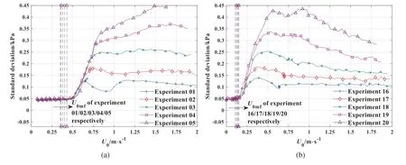
When U0

4.1.1.Empty bed experiment

The number of the empty bed experiment is 00,and the relationships between fan openings,U0and ΔPpare shown in Fig.3.As seen from Fig.3,with an increase in the fan opening,U0and ΔPpcontinue to increase.As mentioned in Section 3.1,in the data processing of other experiments(experiment 01–25),the mapping relationship between ΔPpand U0is needed to calculate the precise ΔP.

4.1.2.Experiments with materials

According to the design of the experimental steps,25 experiments were continuously carried out.Before each experiment,the distribution plate with its screen and filter bag were cleaned and prefluidized at a 50% fan power for 15 minutes to keep the material in a dry and loose state to ensure that all experiments were carried out under the same conditions.Unfortunately,due to unknown interference factors(voltage fluctuations,electromagnetic interference,etc.),portions of the analysis results for experiment 06 do not quite conform to the overall rules.Furthermore,since the experimental conditions cannot be restored perfectly,experiment 06 cannot be performed again.However,since the experimental quantity is large enough,this limitation does not affect the derivation of rules in this study.

Fig.3.U0 and ΔPp at different fan openings of the empty bed experiment(number 00).

The relationship between the fan openings and U0in experiment 07 is shown in Fig.4.It can be seen that after adding material,U0is smaller under the same fan opening compared with the empty bed experiment (number 00).In addition,for experiment 07,U0shows a temporary phenomenon of ceased growth when the fan opening is approximately 35%,which is called the gas velocity platform in this paper.By analyzing the data of other experiments,it was determined that the gas velocity platform is a common phenomenon.The characteristics of the gas velocity platform will be specifically described below.

4.1.3.Characteristics of the gas velocity platform

As shown in Fig.5,the 3rd row and 3rd column of the data in Table 2 are taken to display the regularity of the appearance of the gas velocity platform;the experimental numbers are 11/12/13/14/15 and 03/08/13/18/23,respectively.The lowermost curve in Fig.5(a)(b) is the actual curve,and the upward curves are the results after successively increasing the gas velocity by 0.5 m﹒s-1in order to facilitate observation.Fig.5(a) shows that the lighter the material mass is,the longer the gas velocity platform is,and the earlier the gas velocity platform occurred.Fig.5(b) shows that the smaller the particle size is,the longer the gas velocity platform is.

Fig.4.U0 at different fan openings for experiments 00/07.

Fig.5.U0 at different fan openings of (a) the 3rd row and (b) the 3rd column of experiments in Table 2,the gray area represents the gas velocity platform defined in Section 4.1.3.

According to the experimental design,it can be determined that each row of data can reflect the relationship between the target value and the material mass,and each column of data can reflect the relationship between the target value and the particle size.Therefore,due to the space limitation of the paper,only some of the data (one or two rows,columns of Table 2) will be displayed.There are similar situations below,and the explanation will not be repeated.

The left and right endpoint values (fan opening) of the gas velocity platform of each experiment are determined,as shown by the gray rectangle block in Fig.5 (Method:the horizontal straight line of the estimated average value of the gas velocity platform is shifted upward and downward by 0.02 m﹒s-1,respectively,and the interval of the gas velocity platform is determined by measuring the intersection points of the two shifted lines and the U0curve,which is accurate to 0.1% of the fan opening.Not shown in Fig.5).The experiment without the gas velocity platform is indicated by ‘‘-”,as shown in Table 3.It can be seen from Table 3 that the lighter the material mass is,and the smaller the particle size is,the easier the gas velocity platform appears,and the longer it continues.The cause of the gas velocity platform may be the fan characteristics or the transition of the flow regime,or there may be some more complicated reasons,which needs further exploration.If the fan power is increased in the gas velocity platform,the gas velocity will not increase,which is a phenomenon that should be given attention during actual production.

4.2.Signal analysis

There are two pressure time-series signals obtained in this study,SP1and SP2.Since the gas flow is from the plenum (P1 port)and then gets through the fluidized materials to the fluidization chamber (P2 port),it is obvious that SP2contains more fluctuation information than SP1(signal analysis results proved that).Therefore,in the following sections of signal analysis,only SP2is used to discuss the correspondence between the characteristic values and the influencing factors.

4.2.1.Standard deviation

As shown in Fig.6,the 1st and 4th rows of the data in Table 2 are taken to display the relationship between the standard deviation and the material mass,where the experimental numbers are 01/02/03/04/05 and 16/17/18/19/20,respectively.A series of vertical dotted lines on the left side of Fig.6 represent U0mfof each experiment,and their colors and markers are the same as the curves of corresponding experiments.Since the U0mfvalues of the experiments in the same row are very close,these vertical dotted lines are intensively indistinguishable,so the correspondence between these vertical dotted lines and experiments is labeled with the text in Fig.6.If there are such vertical dotted lines or text labels in the remaining figures,they have the same meaning,and the explanation will not be repeated.

Table 3 Fan opening interval of the gas velocity platform of each experiment

Fig.6 shows that when U0U0mf,the standard deviation rapidly increases with a similar growth rate,indicating that the amplitude of the pressure fluctuation increases.When U0increases to a certain gas velocity,the curves show an inflection point andenter a relatively stable state;the larger the material mass is,the larger the maximum standard deviation is.Many scholars[8,20,21] stated that the standard deviation of pressure fluctuations is positively correlated with bubble size.Since larger bubbles are more likely to be formed when the material mass is larger,so this theory is consistent with the experimental results.As U0continues to increase,the curves in Fig.6(b) decrease at different U0values,and the larger the material mass is,the larger U0of the decreasing point is.

Fig.6.Standard deviation at different U0 values of(a)the 1st row and(b)the 4th row of experiments in Table 2.U0mf values of experiment 01/02/03/04/05 and 16/17/18/19/20 are 0.351/0.360/0.380/0.402/0.430 and 0.108/0.122/0.134/0.142/0.151,respectively.(unit:m﹒s-1).

As shown in Fig.7,the 2nd and 4th columns of the data in Table 2 are taken to display the relationship between the standard deviation and the particle size,and the experimental numbers are 02/07/12/17/22 and 04/09/14/19/24,respectively.Fig.7 shows that the maximum standard deviations of the experiments with different particle sizes are almost the same.In addition,Fig.7(b)shows that after the inflection point,all curves decrease at a certain U0position and that the smaller the particle size is,the smaller U0of the decreasing position is.Since the material mass of Fig.7(a)is too light(2.5 kg),the fluidized states are disordered,so the above phenomenon is not clearly observed in this figure.

The most important characteristic of the standard deviation is that it rises rapidly at U0mf,and this method is often used in actual production to determine that the flow regime changes from fixed bed to bubbling fluidization.In addition,when the material mass is relatively large(>2.5 kg),it can be clearly observed that the standard deviation curves decrease at a certain position after reaching the maximum value.According to the views of many scholars[32,33],U0of the maximum standard deviation is the transition velocity from bubbling fluidization to turbulent fluidization.Therefore,it can be concluded that the smaller the material mass is and the smaller the particle size is,the easier it is to enter the turbulent fluidized state.

4.2.2.Skewness

Fig.7.Standard deviation at different U0 values of(a)the 2nd column and(b)the 4th column of experiments in Table 2.U0mf values of experiment 02/07/12/17/22 and 04/09/14/19/24 are 0.360/0.299/0.208/0.122/0.110 and 0.402/0.332/0.214/0.142/0.129,respectively.(unit:m﹒s-1).

Fig.8.Skewness at different U0 values of(a)the 1st row and(b)the 4th column of experiments in Table 2.U0mf values of experiment 01/02/03/04/05 and 04/09/14/19/24 are 0.351/0.360/0.380/0.402/0.430 and 0.402/0.332/0.214/0.142/0.129,respectively.(unit:m﹒s-1).

As shown in Fig.8,the 1st row and 4th column of the data in Table 2 are taken to display the regularity of the skewness in terms of the material mass and particle size,and the experimental numbers are 01/02/03/04/05 and 04/09/14/19/24,respectively.Fig.8 shows that when U0U0mf,the skewness rapidly rises to the maximum value point and then rapidly drops.Fig.8(a)shows that the maximum value of the skewness increases as the material mass increases,and the U0of the maximum value point is independent of the material mass.Fig.8(b)shows that the maximum value of the skewness is independent of the particle size,and the U0of the maximum value point increases as the particle size increases.

Although the skewness has a relatively clear variation rule,the skewness is very disordered under the condition of a light material mass,and its variation amplitude is too small to be applied to actual production.

4.2.3.Kurtosis

As shown in Fig.9,the 1st row and 4th column of the data in Table 2 are taken to display the regularity of the kurtosis in terms of the material mass and particle size,and the experimental numbers are 01/02/03/04/05 and 04/09/14/19/24,respectively.Fig.9 shows that when U015).When U0>U0mf,the kurtosis rapidly drops to approximately 2.5.

Based on all the experiments,it can be concluded that the variation rule of the kurtosis is that when U0reaches U0mf,the kurtosis decreases from 15 to approximately 2.5,which is independent of both the material mass and particle size.Therefore,the kurtosis can be used as a very simple and reliable method to determine the flow regime.Kurtosis characterizes the sharpness of the probability density function of the signal,indicating that the distribution is very concentrated before the occurrence of fluidization and tends to a normal distribution after that.

4.2.4.Main frequency and absolute power spectrum density

Fig.9.Kurtosis at different U0 values of(a)the 1st row and(b)the 4th column of experiments in Table 2.U0mf values of experiment 01/02/03/04/05 and 04/09/14/19/24 are 0.351/0.360/0.380/0.402/0.430 and 0.402/0.332/0.214/0.142/0.129,respectively.(unit:m﹒s-1).

Fig.10.Main frequency and Pxxa.max at different U0 values of(a)the 1st row and(b)the 4th row of experiments in Table 2.U0mf values of experiment 01/02/03/04/05 and 16/17/18/19/20 are 0.351/0.360/0.380/0.402/0.430 and 0.108/0.122/0.134/0.142/0.151,respectively.(unit:m﹒s-1).

As shown in Fig.10,the 1st and 4th rows of the data in Table 2 are taken to display the relationship between the main frequency,Pxxa.maxand the material mass,and the experimental numbers are 01/02/03/04/05 and 16/17/18/19/20,respectively.Fig.10 shows that when U0U0mf,the main frequency enters a region of continuous growth,and Pxxa.maxalso rapidly rises to the maximum value of approximately 5 Hz-1and then decreases.At this stage,when at a same U0value,the experiment with less material mass has a higher main frequency.The variation rules of Pxxa.maxfor different experiments are similar;in the experiment with larger material mass,the maximum Pxxa.maxvalue is slightly larger,and the U0value corresponding to the maximum Pxxa.maxpoint is also slightly larger.Since Pxxa.maxrepresents the concentration of the signal energy at the main frequency,the experiments with larger material mass can achieve a more stable fluidized state.The experimental observation in this stage shows that the material presented a very regular periodic motion and emitted a very regular sound,and their frequencies were very close to the main frequency of the pressure signal.Therefore,we consider that this dominant signal comes from the material movement,and therefore,we call this dominant signal the material motion signal.As U0continues to increase,the power of a signal with a frequency of 2.5 Hz continues to increase (observed through the corresponding power spectrum image,not shown in this paper),and even in some experiments,the power of the 2.5 Hz signal exceeds that of the material motion signal,resulting in a sudden decrease of the main frequency curve.The lighter the material mass is,the smaller U0of the decreasing position is.The experimental observation in this stage shows that,unlike the former stage,the material motion was disordered and had no obvious periodicity.

Fig.11.Main frequency and Pxxa.max at different U0 values of(a)the 2nd column and(b)the 4th column of experiments in Table 2.U0mf values of experiment 02/07/12/17/22 and 04/09/14/19/24 are 0.360/0.299/0.208/0.122/0.110 and 0.402/0.332/0.214/0.142/0.129,respectively.(unit:m﹒s-1).

As shown in Fig.11,the 2nd and 4th columns of the data in Table 2 are taken to display the relationship between the main frequency,Pxxa.maxand the particle size,and the experimental numbers are 02/07/12/17/22 and 04/09/14/19/24,respectively.Fig.11 shows that the smaller the particle size is,the smaller the U0value of the decreasing position is.It can be seen from the Pxxa.maxcurve that the distances between U0mfand U0of the maximum Pxxa.maxare almost the same.When Pxxa.maxcurve reaches its maximum value,the fluidized bed is in the most simple and stable fluidized state,which is particularly suitable for some production processes that needed to be accurately controlled.

According to Figs.10 and 11,when U0U0mf,in the initial stage,the dominant signal is the material motion signal,and the fluidized state is very simple and stable.With the continuous increase in U0,the power of the 2.5 Hz signal continues to increase,and the fluidized state becomes complex and disordered,which may be related to the turbulent fluidization.In particular,the frequencies of the so called ‘‘2.5 Hz signal”are close to 2.5 Hz in all the experiments (which is why this signal is called the 2.5 Hz signal);this result is independent of both the material mass and particle size.Therefore,the 2.5 Hz signal may be related to the structure and size of the fluidized bed.However,the specific source of the 2.5 Hz signal needs further exploration.

4.2.5.Average cycle frequency

As shown in Fig.12,the 4th row and 2nd column of the data in Table 2 are taken to display the regularity of the average cycle frequency in terms of the material mass and particle size,and the experimental numbers are 16/17/18/19/20 and 02/07/12/17/22,respectively.Eq.(6) shows that the average cycle frequency can be regarded as the average frequency of all components of the signal,so the variation trend of the average cycle frequency curve is similar to that of the main frequency curve,but the former is smoother.When U0U0mf,the curves enter a growth state.Fig.12(a) shows that the experiment with less material mass has a higher average cycle frequency.As U0continued to increase,some of the curves remain relatively stable,and some curves show a decrease,reflecting that the power of the 2.5 Hz signal increases gradually.Fig.12(a)(b)shows that the lighter the material mass is and the smaller the particle size is,the smaller the U0value of the decreasing position is.

Both the average cycle frequency and the power spectrum are frequency observation methods of the fluidized state,and the values obtained by the two methods have similarities and differences.The frequency observation methods are mainly used to determine the components of the signals and their respective intensities,and then to analyze the fluidized state.According to the results,the curves of the two methods were both confused and difficult to apply to actual production.To solve this problem,a new analysis method is proposed,which can easily determine the fluidized state in the fluidized bed,as described below.

4.2.6.Combined analysis of the main frequency and average cycle frequency

The main frequency characterizes the frequency of the most powerful signal component,while the average cycle frequency characterizes the average frequency of the various signal components.If the two frequencies are close,it can essentially be explained that there is only one main signal component in the fluidized bed at this time,and the fluidized state is relatively stable.It is generally believed that the product quality is stable and controllable under a stable fluidized state,so it is important to accurately determine the fluidized state during actual production.The specific calculation method proposed in this paper is to divide the main frequency by the average cycle frequency,as follows:

where Q is the characteristic value of the fluidized state,fmis the main frequency obtained by the power spectrum,and fcis the average cycle frequency.

As shown in Fig.13,the 1st and 4th rows and the 2nd and 4th columns of the data in Table 2 are taken to display the regularity of Q in terms of the material mass and particle size,and the experimental numbers are 01/02/03/04/05,16/17/18/19/20,02/07/12/17/22,and 04/09/14/19/24,respectively.For each U0,Q is calculated and depicted as a curve with U0as the abscissa.According to the above,when the two frequencies are close,the fluidized state is relatively stable.In other words,when Q approaches 1,the fluidized state is relatively stable.Fig.13 shows that,when U0>U0mf,as U0grows,the Q curves quickly approach the line y=1 (horizontal dotted line in the figure),then remain stable for a time,and then deviate from the line y=1.

Fig.12.Average cycle frequency at different U0 values of(a)the 4th row and(b)the 2nd column of experiments in Table 2.U0mf values of experiment 16/17/18/19/20 and 02/07/12/17/22 are 0.108/0.122/0.134/0.142/0.151 and 0.360/0.299/0.208/0.122/0.110,respectively.(unit:m﹒s-1).

Fig.13.Q at different U0 values of(a)the 1st row,(b)the 4th row,(c)the 2nd column,and(d)the 4th column of experiments in Table 2.The gray areas represent the stable fluidized zone defined in Section 4.2.6.U0mf values of experiment 01/02/03/04/05,16/17/18/19/20,02/07/12/17/22,and 04/09/14/19/24 are 0.351/0.360/0.380/0.402/0.430,0.108/0.122/0.134/0.142/0.151,0.360/0.299/0.208/0.122/0.110 and 0.402/0.332/0.214/0.142/0.129,respectively.(Unit:m﹒s-1).

In Fig.13,two lines of y=1.02 and y=0.98 are drawn in each coordinate system (not shown in figure).By measuring the intersection points of the above two lines and the Q curve,the gas velocity interval where Q closest to 1 is calculated,which is accurate to 0.001 m﹒s-1.This interval is defined as the stable fluidized zone,as shown by the gray interval in Fig.13.The measuring results are listed in Table 4(As mentioned in Section 4.1.2,since the stable fluidized zone of experiment 06 cannot be measured,it is replaced by‘‘-”).Fig.13(c)(d)shows that the larger the particle size is,the larger the left and right endpoint values are,and the smaller the interval length is (only experiment 02 does not conform to this rule).However,the effect of the material mass on the stable fluidized zone is not very clear,as shown in Fig.13(a)(b).In this study,the experimental quantity was limited,and the gas velocity had a relatively large control interval,and the data screening,processing and analysis methods also had an optimization space.Thus,the summary of rules was not sufficient.In later research,these aspects will be optimized to obtain quantitative rules.During actual production,the materials designated by the process parameters can be tested in advance,and the corresponding stable fluidized zones can be analyzed.Controlling the gas velocity within the range of the stable fluidized zone during actual production ensures that the fluidized bed consistently remains in a stable fluidized state.

Table 4 Gas velocity interval of the stable fluidized zone of each experiment

5.Conclusions

In this work,the pressure fluctuations of the negative pressure conical pharmaceutical fluidized bed are studied,and various mathematical analysis methods (time domain analysis and frequency domain analysis) are used to identify the correspondence between the characteristic values obtained by these methods and the influencing factors(material mass and particle size)or the fluidized state.

The conclusions of this study can be summarized as follows:

1.The phenomenon where U0temporarily stops growing is called the gas velocity platform.The lighter the material mass is and the smaller the particle size is,the more easily the gas velocity platform appears,and the longer it continues.If the fan power is increased in the gas velocity platform,the gas velocity will not increase.

2.As U0increases,when U0reached U0mf,the standard deviation rapidly increases while the kurtosis value rapidly decreases,indicating that the flow regime changes from fixed bed to bubbling fluidization.As U0continues to increase,standard deviation decreases at certain U0values,which means that the bed enters the turbulent fluidization.The smaller the material mass is and the smaller the particle size is,the easier it is to enter the turbulent fluidized state.The maximum standard deviation value increases as the material mass increases,so the standard deviation can be used as an auxiliary monitoring tool for the material mass.The variation rule of the kurtosis is independent of both the material mass and particle size.

3.By analyzing the results of the power spectrum and the average cycle frequency,it can be concluded that when U0>U0mf,in the initial stage,the dominant signal is the material motion signal,and the fluidized state is very simple and stable,and the flow regime is bubbling fluidization at this time.With the continuous increase in U0,the power of the 2.5 Hz signal continues to increase,and the fluidized state becomes complex and disordered,which may be related to the turbulent fluidization.The specific source of the 2.5 Hz signal needs further exploration.

4.The method of dividing the main frequency by the average cycle frequency,which is proposed in this paper,can conveniently determine the current fluidized state.Furthermore,the stable fluidized zone can be obtained by this method.Controlling the gas velocity within the range of the stable fluidized zone during actual production ensures that the fluidized bed consistently remains in a stable fluidized state.The larger the particle size is,the larger the left and right endpoint values of the stable fluidized zone are,and the smaller the interval length is.The quantitative rules of the stable fluidized zone require further exploration.

Declaration of Competing Interest

The authors declare that they have no known competing financial interests or personal relationships that could have appeared to influence the work reported in this paper.

Acknowledgements

This work was supported by the National Standardization Project of TCM(ZYBZH-C-TJ-55)and National Science and Technology Major Project(2018ZX09201011-002).We thank American Journal Experts (AJE) for English language editing.

Nomenclature

d window function

fcaverage cycle frequency,Hz

fmmain frequency obtained by the power spectrum,Hz

K kurtosis of the time-series signal

M length of each segment

N total point number of the time-series signal

Ncnumber of times the time domain curve passes through its average value during a given time

Pxtaverage power of xt(n),Pa2

Pxxpower spectrum density of xt(n),Pa2﹒Hz-1

Pxxaabsolute power spectrum density of xt(n),Hz-1

Pxxa.maxmaximum value of Pxxa,Hz-1

ΔP pressure drop between the top and bottom sections of the material,Pa

ΔPppressure drop at the gas distribution plate,Pa

Q characteristic value of the fluidized state

S skewness of the time-series signal

Sfflowrate time-series signal,L﹒min-1

SP1average value of SP1,Pa

SP2average value of SP2,Pa

t measurement time of the signal,s

U normalization factor

U0gas average velocity at the bottom section of the conical cylinder,m﹒s-1

U0mfminimum fluidization velocity at the bottom section of the conical cylinder,m﹒s-1

W material mass,kg

x(n) original time-series signal

xt(n)processed signal used to calculate Pxx

σ standard deviation,Pa