WU He, YU Huaming, FANG Yizhou, ZHOU Qingwei, ZHUO Fengxuan,and KELLY Ryan M.

Assessment of the Tidal Current Energy Resources and the Hydrodynamic Impacts of Energy Extraction at the PuHu Channel in Zhoushan Archipelago, China

WU He1), YU Huaming2), *, FANG Yizhou1), ZHOU Qingwei1), ZHUO Fengxuan3),and KELLY Ryan M.4)

1) National Ocean Technology Center, Tianjin 300112, China 2) College of Oceanic and Atmospheric Sciences, Ocean University of China, Qingdao 266100, China 3) Southern Marine Science and Engineering Guangdong Laboratory, Zhuhai 519082, China 4) Rykell Scientific Editorial, Placentia, CA 92871, USA

An unstructured model FVCOM (The Unstructured Grid Finite Volume Community Ocean Model) with sink momentum term was applied to simulate the tidal current field in Zhoushan Archipelago, China, with focus on the region named PuHu Channel between Putuo Island and Hulu Island. The model was calibrated with several measurements in the channel, and the model performance was validated. An examination of the spatial and temporal distributions of tidal energy resources based on the numerical simulation revealed that the greatest power density of tidal energy during spring tide is 3.6kWm−2at the northern area of the channel. Two parameters were introduced to characterize the generation duration of the tidal array that causes the temporal variation of tidal current energy. The annual average available energy in the channel was found to be approximately 2.6MW. The annual generating hours at rated power was found to be 1800 h when the installed capacity of tidal array is approximately 12MW. A site for the tidal array with 25 turbines was selected, and the layout of the array was configured based on the EMEC specifications. Hydrodynamic influence due to the deployment of the tidal array was simulated by the modified FVCOM model. The simulation showed that the tidal level did not significantly change because of the operation of the tidal array. The velocity reduction covered a 2km2area of the downstream the tidal array, with a maximum velocity reduction of 8cms−1at mid-flood tide, whereas the streamwise velocity on both sides of the farm increased slightly.

tidal current energy; resources assessment; numerical simulation; hydrodynamic effects

1 Introduction

Ocean energy is promoted by governments as a form of renewable energy that will aid in the mitigation of climate change and contribute to energy security in the relevant countries. Many coastal countries are developing specific strategies and plans for extracting ocean energy and committing national funding toward ocean energy research and deployment (The Executive Committee of OES, 2019). As one form of renewable energy, tidal current energy extraction is a feasible energy source with the advantages of High Technical Readiness Level of Level 7–8 (Mofor, 2014), no land occupation, predictable, and relatively low environmental impact compared to tidal range energy extraction (Brooks, 2006). Moreover, because the sites with much tidal energy potential are usually near large coastal cities with great electricity demand, trans-mission loss is reduced.

The Zhoushan Archipelago, located in the eastern Chinese province of Zhejiang, contains hundreds of channels that are potential sites for tidal energy extraction. A fundamental method for tidal energy assessment is the measurement of tidal current data. A comprehensive study assessed over 130 water channels at the national level in 1989 based on the tidal data from a marine atlas; the results of the study showed that the power density of tidal energy in most of their water channels is 15–30kWm−2, with particularly high power densities in Jintang Channel, Guishan Channel, and Xihou Channel in the Zhoushan Archipelago (Wang and Lu, 2009). Wang(2010) discussed the characteristics of tidal current energy based on measured tidal current at 5 sites in the Gaoting Channel and 8 sites in the Guanmen Channel; he also used the Technical Available Resource method of Farm and Flux to reveal that the utilizable tidal power is 4.67–5.31MW in the Gaoting Channel and 7.92–9.37MW in the Guanmen Channel. However, these results may overestimate the energy potential because it is hard to correlate the level in the whole channel with the exited power density at a specific point.

With the development of numerical simulation, ocean modeling based on the Navier-Stokes equations has been increasingly applied to the assessment of tidal energy in recent years as it can provide substantially more ‘field’ tidal current data to describe the elaborate and accurate spatial and temporal distribution of tidal energy. The tidal current energy levels of eight channels in this archipelago with maximum currents greater than 2.5ms−1wereanalyzed based on an ocean model. This study also showed that the total tidal current energy of the important watercourse can be 1400MW (Hou, 2014). A more comprehensive assessment of tidal energy over this region was subsequently carried out using ocean modeling; the assessment showed that the theoretical annual average potential of tidal energy resources in Zhoushan Archipelagoof58mainchannelsisapproximately3950MW,whichis almost equal to the capacity of two Three Gorges Power Stations (Luo, 2017). A study of Deng and coworkers (Deng, 2020) provided insight into the environmental impacts of a large-scale tidal arraya numeri- cal investigation in Zhoushan waters, with focus on the changes in current velocity, tidal elevation, and sediment transport. The hydrodynamic responses, especially after deployment of the tidal turbine array, are still not fully understood and may give rise to significant effects on the marine environment. For example, the tidal energy utilization may affect numerous environmental variables, such as the tidal regime, hydrodynamics, suspended and sediment transport, and water quality(Couch and Bryden, 2004;Blunden and Bahaj, 2007; Ramos, 2013; Nash, 2014; Bai, 2016; Chen and Liu, 2017; Lin, 2017).

Among the potential sites for the execution of tidal current energy extraction, the one that lies between Putuoshan Island and Huludao Island (hereby named the PuHuChannel) is one of the most plausible sites. Large-scale operation of dozens of tidal turbines array can become a long-term, sustainable renewable energy source for Zhou- shan City. Zhang(2020a) carried out numerical experiments on tidal energy extraction in the PuHu Channel using the two-dimensional OpenTidalFarm model and investigated the optimal array layout for energy extraction; the hydrodynamic impact of large-scale (, 115 turbines) tidal energy extraction in this channel was examined by Zhang(2020b)the 3-D hydrodynamic model with turbine representation based on the blade element method.

In this paper, an assessment of the tidal current energy levels over the Zhoushan Archipelago, with focus on the PuHu Channel, is presented in detail based on FVCOM (The Unstructured Grid Finite Volume Community Ocean Model, Chen, 2003, 2006). In contrast to previous studies, a resource assessment of the tidal stream energy in the PuHu Channel is carried out first to determine the suitable capacity of the tidal array. Next, the representation of the tidal turbine is integrated into this ocean modelmomentum sink terms. The impacts of the tidal arrays on the hydrodynamic conditions are then investigated with the wake characteristics of the tidal current turbines and the wake recovery in the downstream of devices; the results of the investigation could be taken as a scientific reference for the future design of a tidal power demonstration project.

2 Methods

2.1 Governing Equations

FVCOM is an ocean modeling software that can simulate the water surface elevation, velocity, temperature, salinity, sediment transport, and water quality constituents. With unstructured triangular cells in the horizontal plane and a sigma-stretched coordinate system in the vertical direction, this model could represent optimally the complex horizontal geometry and the bottom topography of estuaries. The unstructured-grid and finite-volume approaches employed in the model provide geometric flexibility and computational efficiency that are well suited for simulation of tidal energy extraction, which requires higher grid resolution in the region of a tidal turbine array, nestled within the larger model domain. Finer grid resolution is mandatory for the tidal turbine array surroundings to account for shifts in flow fields, the dissipation of kinetic energy, and downstream wake signatures.

FVCOM is governed by a set of primitive equations representing momentum, continuity, temperature, salinity, and density. The Navier-Stokes (N-S) equations solved by the numerical model in the original Cartesian coordinate form are depicted as (- and- directions displayed):

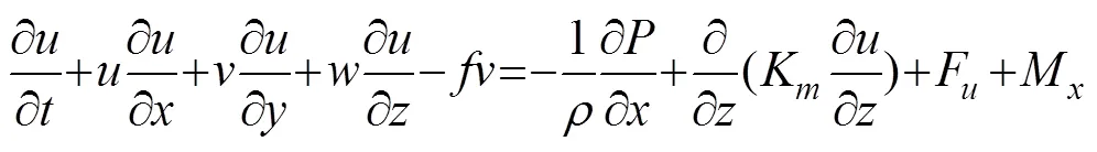
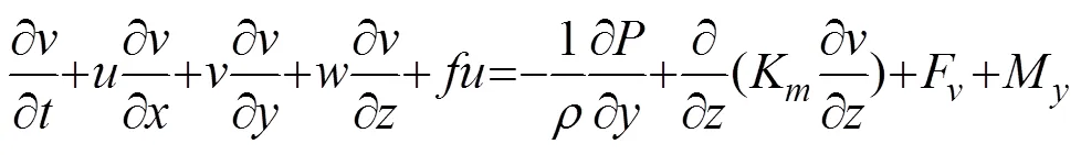
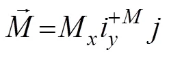
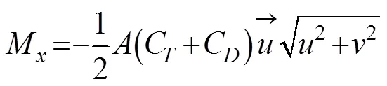
whereis the time;,, andare the east, north, and vertical axes in the Cartesian coordinate system, respectively;,, andare the three velocity components in the,, anddirections, respectively;0is the water density;is the pressure arising from the sea surface and the water;is the non-hydrostatic pressure;is the Coriolis parameter; andKis the vertical eddy viscosity coefficient.FandFrepresent the horizontal momentum terms.MandMrepresent the additional horizontal momentum terms from tidal turbines specified in the later section. The total water column depth is=+, whereis the bottom depth (relative to=0), andis the height of the free surface (relative to=0).

The-coordinate transformation is used in the vertical direction to obtain a smooth representation of the bottom topography irregularities and is defined as:

where the value of sigma ranges monotonically from=−1 (bottom) to=0 (surface). Interestingly, ocean models differ from atmospheric models in that the-coordinates are normalized, varying from=1(surface) to=0 (top of atmosphere),

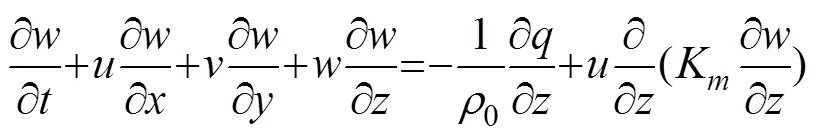
The surface and bottom boundary conditions for,, andare:

where=0.4 is the von Karman constant, and0is the bottom roughness parameter. FVCOM features a wide choice of ocean turbulence closure models for the parameterization of the vertical eddy viscosity and the vertical thermal diffusion coefficient; furthermore, an updated version of the MY-2.5 model used in this model has been testified successfully in many cases.

2.2 Parameterization of Tidal Current Turbines

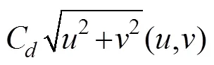
One important aspect of the study is the modeling of the hydrodynamic changes from a turbine array acting on the water column. In fact, the extraction process is extremely complex because the fluid that has passed the turbines becomes rotational and attached to the boundary layer at high Reynolds number flow, and the structure of the wake immediately behind the body depends strongly on the body’s geometry. To simplify the process of macro effect on the hydrodynamic environment, the following three approaches are applied widely: the bottom friction approach, the momentum sink approach, and the blade ele-ment actuator disk approach (Chen, 2014). Among these approaches, the momentum sink approach is the most popular method; this method represents the loss of momentum due to tidal energy extraction by adding a termto the momentum equations(Ahmadian and Falconer, 2012;Chen, 2013; Chen, 2014; Sanchez, 2014; Wu, 2017).

3 Study Area and Model Configuration

3.1 Study Domain

The PuHu Channel is located 6km (latitude-wise) to the east of Zhoushan Island and is approximately 3.0km by 2.0km, with an orientation of northwest–southeast (Fig.1). A small isle splits the north exit into two pathways; the eastern and western pathways are 1.2km and approximately 1.0km in length, respectfully. The depth of the PuHu Channel is between 20m and 60m, the bathymetric gradient along coastlines is steep, and the central area of the bathymetry is relatively flat. The flooding and ebbing directions are northwestward and southeastward along the coast, respectively.

3.2 Model Configuration

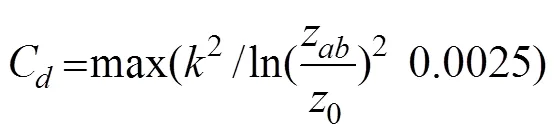
This study used an unstructured-grid coastal ocean model with a resolution refinement for the PuHu Channel region. The model covers the entire Hangzhou Bay, the grid size of which is from approximately 2.5km along the open boundary to 10 m around the potential site for tidal turbines array at the north of the channel in order to describe it elaborately (Fig.2). Ten vertical layers of uniform thickness were specified in the water column using the sigma-stretched coordinate system. The Smagorinsky scheme for horizontal mixing and the MY-2.5 turbulent closure scheme for vertical mixing were used in this model. The bottom friction is described by the quadratic law with the drag coefficient determined by the logarithmic bottom layer as a function of the bottom roughness. A bottom friction coefficient of 0.0025 and a bottom roughness of 0.001m were used in the model. The model run time step was 0.2s. Open boundary conditions for the model were specified at the east side of Hangzhou Bay using 9 harmonic tidal constituents (, S2, M2, N2, K2, K1, P1, O1, Q1, and M4) provided by the global tidal model TPXO7.2. The dominant tidal constituents are the principal semi-diurnal tide M2and the principal diurnal tide K1. The Qian-tang River inflows were assumed to be 697m3s−1, and other geophysical factors (such as wind field, evaporation, atmospheric precipitation, and bottom freshwater) were neglected.

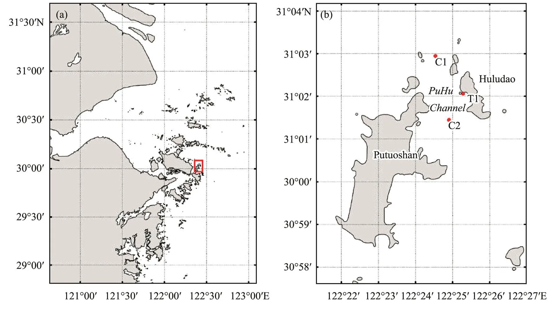
Fig.1 Location of the PuHu Channel (red box) which is between Huludao Island and Putuoshan Island in the Zhoushan Archipelago, with the locations of the tidal current observation stations, C1 and C2, and the tidal elevation gage, T1 (red dots).

Fig.2 Model mesh of the Zhoushan Archipelago (a) and the PuHu Channel (b).

3.3 Model Validation

The model was validated by observation data at one tide gauging station and two tidal current stations shown in Fig.2. The simulation period, which lasted for 31 days starting from 1st to 31st August, 2014, includes two spring-neap cycles. Fig.3 and Fig.4 show the comparison between model result and measure data on surface elevation and depth-averaged current speed, respectively. It can be seen that the water level from the model predictions follows the observed data closely, except for a couple of centimeters of underestimation on a few occasions at high tides. The current speed predictions are in reasonable a- greement with the measured data, with a RMSE of 15cms−1at the T1 station and 17cms−1at the T2 station, except that the magnitude of the current speed at the mid-flooding moment was slightly underrated. This discrepancy could be relatedtothecomplexbathymetryandmeteorologicalforce that might not be represented accurately in the model.

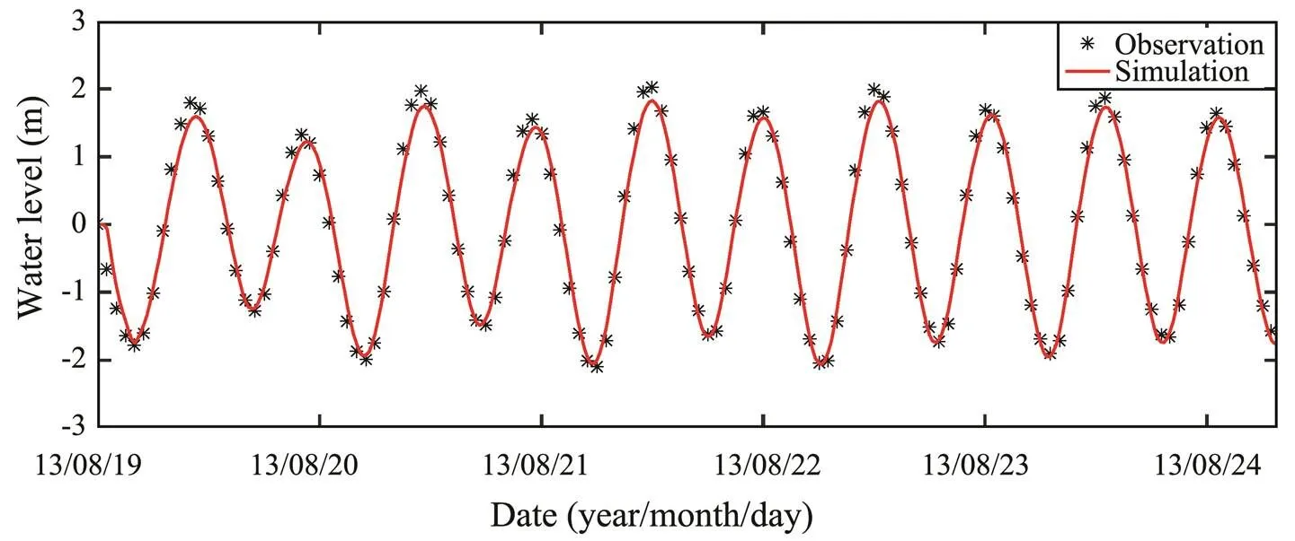
Fig.3 Validation of surface elevation at the tidal elevation gauging station, T1 (refer to Fig.1 for mapped tidal gage station location, RMSE=12cm).

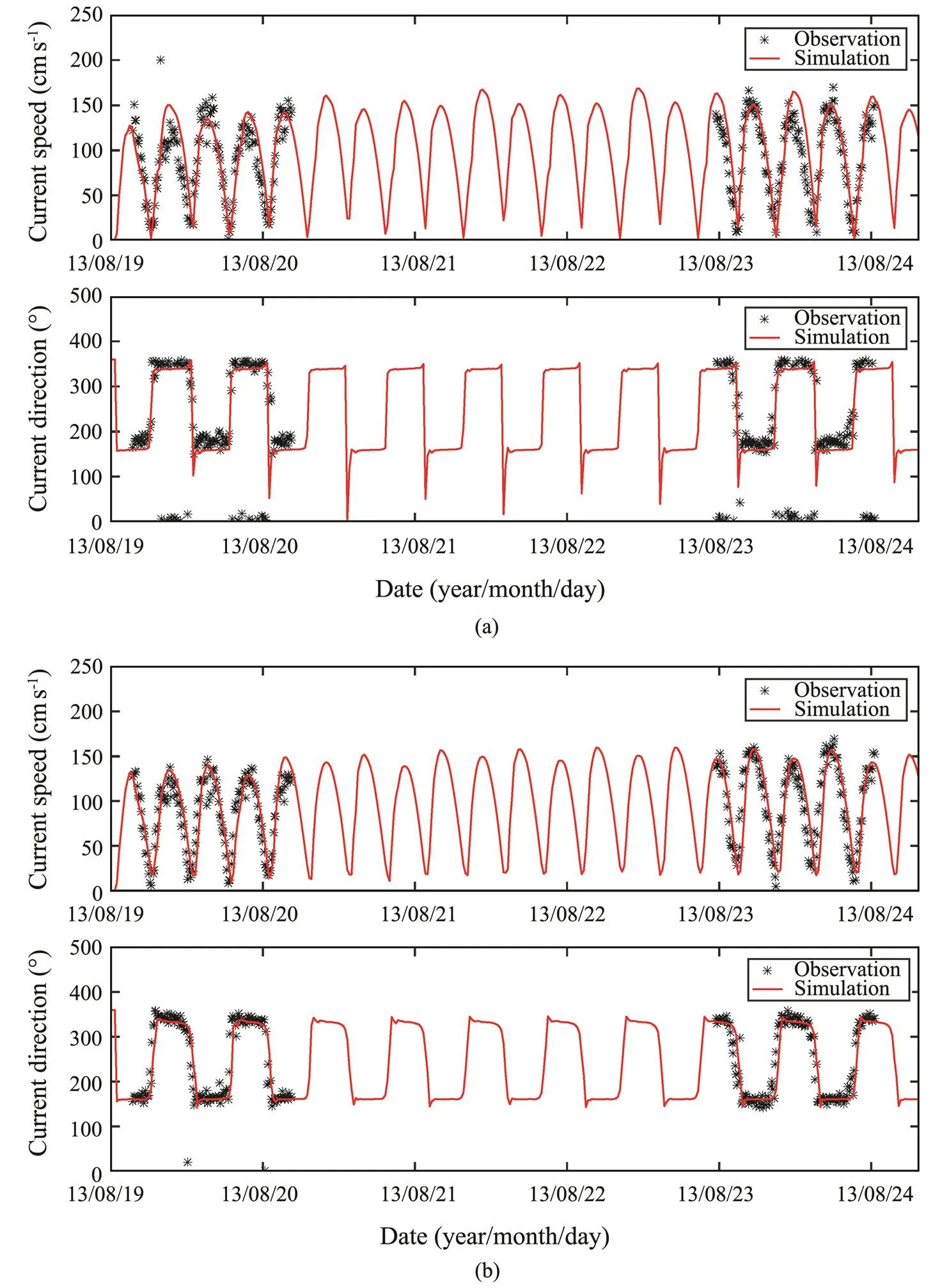
Fig.4 Comparison of the measured (black stars) and the simulated (red lines) tidal current speed and direction at two tidal current observation stations T1 (a) and T2 (b) (refer to Fig.1 for mapped tidal current observation station locations).

4 Characteristics of Tidal Current Energy

4.1 Distribution of Current and Power Density

Because of the good model validation results described above, the model was used to calculate the unaltered tidal flow velocities over the channel. Fig.5 depicts the flow velocities at mid-flood and mid-ebb on a spring tide of 23rd August, 2013, which indicates there are 3 sites with stronger flow at the north, middle, and south of the channel. The maximum speeds in the three areas is 2.1ms−1, 2.3ms−1, and 1.8ms−1during the flooding period, and they are 2.1ms−1, 1.9ms−1, and 1.7ms−1during the ebb period. The main velocity direction along the coastlines of islands is northwest-southeast. It can also be observed that the velocity decreases from the middle of the channel to the coastline.

It is obvious that tidal asymmetry exists in the channel, with the flood tide being stronger than the ebb tide. In this case, this asymmetry can be caused by the different layout of the estuary at different tidal levels or by the distortion of the tidal wave as it propagates over the coastal shelf, as suggested by Ramos(2013).

The tidal current power density calculated from the vertically averaged currents has a similar pattern with tidal current because of the cubic relationship (Fig.6). The maximum power densities at 3 potential sites (Fig.7a) mentioned above are approximately 3.4kWm−2, 3.6kWm−2, and 3.1kWm−2at mid-flood tide and 2.5kWm−2, 2.2kWm−2, and 1.8kWm−2at mid-ebb tide.

Fig.5 Distribution of tidal current at mid-flood (a) and mid-ebb (b) in the PuHu Channel, presented in velocity vectors (black arrows) and speed magnitude (background colors).

Fig.6 Distribution of tidal current energy power density at mid-flood (a) and mid-ebb (b) in the PuHu Channel.

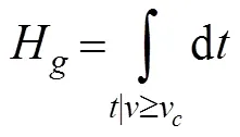
4.2 Distribution of Generation Duration

Therearetwokeyparameters,‘Annualgenerationhours’ (H) and ‘Annual generation hours at rated power’ (H), adopted by the Chinese wind power industry that describe the power generation duration of wind turbines (National Development and Reform Commission, 2004). Similarly,HandHcan also be introduced for tidal energy sources to describe power generation (Eqs. (11)–(12)). The formerHdefines the working time of a tidal turbine in one year, andHdenotes the power generation hours with the rated power in one year,, the total annual energy production divided by the rated power. Fig.7 describes the distribution ofHandHover the PuHu Channel, both of which have a rather similar trend. There are also 3 peaks in the middle of the channel. The highestHreaches 5500h, whereas the highestHis only approximately 2000h. Considering 1800h(H) as the economic value for tidal energy utilization, the area whereHis greater than 1800h is approximately 2.1km2in the channel.

whereHis the annual generation hours;is the time;is the current speed;vis teh cut-in current speed;vis the current speed for the turbine at rated power;His the annual generation hours at the rated power.

Fig.7 Distribution of Hg (a) and Hr (b) of tidal energy in the PuHu Channel.

4.3 Extractable Power Output

Estimation of the energy potential for a specific area is critical to the development of tidal energy sources. An easy method for assessing the potential used broadly named FLUX was used to calculate a certain percentage of the kinetic energy flux through the undisturbed channel, as it only requires measurements of tidal currents and a cross-sectional area that is expressed with Eq. (13)–(14) (Legrand, 2009).

The annual average available poweravailis the product of the power flux passing through the site and the significant impact factor (). Previous work by Black and Veatch in conjunction with Robert Gordon University (Bryden, 2007) suggested that the SIF will be dependent on the type of site. The SIF represents the percentage of the total resource at a site that can be extracted without significant economic or environmental effects. Extraction percentage is set to 15% in this paper according to the suggestions of EPRI (Hagerman, 2006).

The power flux (FLUX) passing through a certain section of a channel can be calculated using:

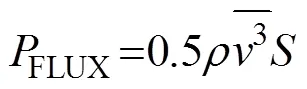
whereis the water density;is the current speed;is the area of delegate section ranging from 0.5km2to 0.6km2.

The annual available power gradually increases from the north exit to the south exit of the channel because of the different areas of a typical section and the different distributions of current speed. The maximumavailis 3.23MW at the north exit, whereas the minimum value is 1.98MW (Fig.8); the average value of 2.60MW along the channel can be considered as the available potential of this channel. Note that the results cannot be used to calculate the power capacity and turbine number of a tidal farm, as it is annually averaged.

TakingHas 1600h according to the distributions in Fig.7, the capacity of the tidal array at rated power can be simplified and be calculated from the product ofavailand the quotient of hours in one year divided byH(Eq. (15)),, 11.40MW.

5 Hydrodynamic Influence of Tidal Array

5.1 Tidal Turbine Selection

According to the previously presented tidal energy resource characteristics and the bathymetry and morphology of the PuHu Channel, a 25-turbine tidal array with a rated power of 12MW is added to the model.

5.2 Site Selection and Layout of Tidal Array

A suitable region for the tidal array not only has much energy potential but also other physical characteristics that allow for the construction of the farm. Several rules employed for siting of a tidal array include:

1) The maximum current velocity should be >2.0ms−1(Khan and Bhuyan, 2009), the water depth should be about20–30m, and the distance to the coastline should be not more than 2.0km.

2) The region should not conflict with navigation, anchorage, oil-gas pipe route, undersea cables, marine protected areas,

3) The wake effects between the turbines should be minimized.

4) The demonstration region should be suitable for the transportation and setup of the tidal turbines and have sufficient area to conduct turbine testing.

Fig.8 Location of the tidal array chosen for the tidal energy extraction points. Note the staggered turbine configuration aligned in the tidal current direction and the linear alignment orthogonal to the current direction. Turbines are equispaced (i.e., 20d, 10d) in their respective directions.

Based on the above criteria and the spatial and temporal distributions of tidal current energy resources, the appointed area of approximately 0.2km2with 0.5km×0.4km and the average depth of 22m were selected on the north of the channel, as shown in Fig.8a. In order to minimize the effects of downstream wake, the lateral spacing between devices (the distance between axes) is set to 5 times the rotor diameter (5), and the downstream spacing is set to 10 times the rotor diameter (10) (Fig.8) (Legrand, 2009).

5.3 Impact on Hydrodynamic Environment

5.3.1 Water level

Fig.9 illustrates the influence of the tidal array on water level, quantified by the difference of the water level before and after the installation of the tidal array at mid-flood tide and mid-ebb tide. As Fig.9a shows, the water level increases in the southern part of the channel at the mid-flood tide due to the hindrance of turbines array. The maximum range of water level variation is just approximately 0.18cm, but dramatic changes from −0.15cm to 0.16cm appear at the south of the isle in the northern exit, possibly due to the pressure drop caused by the turbines. At the mid-ebbing tide, the water level increases in a very small range at the north of the channel. There is a round-shaped area that appears south to the tidal array, and the range of increase is approximately 0.1cm. In general, the effects on the water level are insignificant and can be neglected in practice. Note that the differences were calculated from instantaneous water levels, which might produce array introduced phase-lag.

5.3.2 Tidal current

As indicated in the previous section, the presence of the tidal array alters the flow, thereby affecting the power density distributions. The differences in the current speed at mid-flood and mid-ebb of a mean spring-tide with and without the tidal array, respectively, are shown in Figs.10aand b. It is apparent that the impacts of the operation of the tidal array are significant, with a reduction in the tidal speed of 8cms−1at both mid-flood and mid-ebb tide. The current difference can be distinguishable even a few kilometers away from the farm. Furthermore, there is an increase in the current velocity on both sides of the tidal array caused by the blockage effect (Chen, 2014).

Fig.11 shows the temporal variation of current speed without turbines and the current speed difference around turbine No. 22. The speed difference changes as a sine curve along tidal process against the original tidal current speed. During a flooding and ebbing process, the maximum difference appeared at the mid-flooding tide and mid-ebbing tide, and the difference trend gradually increases from neap tide to spring tide in the neap-spring cycle. Generally, the speed difference caused by the turbines is negligible, as it is considerably smaller compared to the background current velocity.

Fig.9 Change in water level at mid-flood tide (a) and mid-ebb tide (b) due to the installation of the tidal array.

Fig.10 Current speed difference at mid-flood with the tidal array installed (a) and mid-ebb without the tidal array installed (b).

Fig.11 Current speed difference from neap tide to spring tide at Turbine No. 22.

5.3.3 Impacts on tidal residual current

As one part of the offshore general circulation, tidal residual (tidally averaged) currents govern the net exchange of material with the adjacent coastal area and are therefore of great importance for the health of the marine ecosystem (Garel and Ferreira, 2013). Fig.12a depicts the distribution of the tidal residual field before the operation of the tidal array. Overall, the residual speed is less than 0.03ms−1and is comparably slow on almost the entire area of this channel. However, there are still several sites on which the residual speed is greater than 0.06ms−1; these sites are distributed at the capes of Putuo Island and Hulu Island, and the strongest residual current is approximately 0.15ms−1, which occurs at the southwestern cape of Hulu Island.

Fig.12 shows the spatial distribution of the difference between two modeling scenarios (with or without the tidal array). It can be seen that the current increase occurs at the southern part of tidal array, whereas a decrease occurs at the northern part after the deployment of the tidal array; however, there is no significant variation in the channel. The maximum change with and without turbines appears at the downstream area of the tidal farm during flooding tide and ebbing tide, with a value of approximately 2mms−1, and the other area of the channel is less than 1mms−1.

Fig.12 Temporal averaged tidal residual current without the operation of the tidal array (a) and distribution of the difference in speed (b).

6 Conclusions

A coastal ocean numerical model FVCOM was refined and applied to simulate the hydrodynamic conditions and verified against measured data in the PuHu Channel, Zhou-shan Archipelago. The validated model was then used to estimate the tidal current energy resources of this channel.

The modeling results revealed that the PuHu Channel has 3 sites where the tidal velocities at the mid-flooding tide of a spring tide are over 1.8ms−1. The highest power density, 3.6kWm−2, was found at the central area of the PuHu Channel during the flooding tide, and the highest power density of 2.5kWm−2was found at the west coast of the channel during the ebbing tide. The spatial distributions of the generation duration,HandH, were found to be similar to a power density with 3 peaks, and the maximums ofHandHlocated in the middle of the PuHu Channel reached to 2000h and 5500h, respectively.

The ocean model was modified to simulate the impacts of tidal turbines by adding a sink momentum term to the governing momentum equations. The model results demonstrated that the tidal array would not cause noticeable changes in the water level, with changes of less than 0.2cm. The maximum decrease of the tidal current due to the operation of the tidal array is 8cms−1at both mid-flood and mid-ebb tide in the tidal farm, but the increased velocities on both sides of the array result in the blockage effect. Moreover, the maximum change of tidal residual caused by the introduction of the tidal array that appears at the downstream area of tidal farm during flooding tide and ebbing tide is approximately 2mms−1, and the other area of the channel is less than 1mms−1; such changes are negligible in practice.

Acknowledgements

This work was supported by the National Key R&D Program of China (Nos. 2019YFE0102500, 2019YFB1504401, 2019YFE0102500 and 2016YFC1401800). The au- thors would like to thank the FVCOM Development Group for their modeling support.

Ahmadian, R., and Falconer, R. A., 2012. Assessment of array shape of tidal stream turbines on hydro-environmental impacts and power output., 44: 318-327, https://doi.org/10.1016/j.renene.2012.01.106.

Bai, G., Li, W., Chang, H., and Li, G., 2016. The effect of tidal current directions on the optimal design and hydrodynamic performance of a three-turbine system., 94: 48-54, https://doi.org/10.1016/j.renene.2016.03.009.

Blunden, L. S., and Bahaj, A. S., 2007. Effects of tidal energy extraction at Portland Bill, southern UK predicted from a numerical model.. Porto, Portugal.

Brooks, D. A., 2006. The tidal-stream energy resource in Passamaquoddy-Cobscook Bays: A fresh look at an old story., 31 (14): 2284-2295, https://doi.org/10.1016/j.renene.2005.10.013.

Bryden, I. G., Couch, S. J., Owen, A., and Melville, G., 2007. Tidal current resource assessment., 221 (2): 125-135, https://doi.org/10.1243/09576509JPE238.

Chen, C., Beardsley, R. C., and Cowles, G., 2006. An unstructured-grid, finite-volume coastal ocean model (FVCOM) system., 19 (1): 78-89, https://doi.org/10.5670/oceanog.2006.92.

Chen, C., Liu, H., and Beardsley, R. C., 2003. An unstructured grid, finite-volume, three-dimensional, primitive equations ocean model: Application to coastal ocean and estuaries., 20 (1): 159-186, https://doi.org/10.1175/1520-0426(2003)020<0159:AUGFVT>2.0.CO;2.

Chen, W. B., and Liu, W. C., 2017. Assessing the influence of sea level rise on tidal power output and tidal energy dissipation near a channel., 101: 603-616, https://doi.org/10.1016/j.renene.2016.09.024.

Chen, W. B., Liu, W. C., and Hsu, M. H., 2013. Modeling evaluation of tidal stream energy and the impacts of energy extraction on hydrodynamics in the Taiwan Strait., 6(4): 2191-2203, https://doi.org/10.3390/en6042191.

Chen, Y., Lin, B., and Lin, J., 2014. Modelling tidal current energy extraction in large area using a three-dimensional estuary model., 72: 76-83, https://doi.org/10.1016/j.cageo.2014.06.008.

Chen, Y., Lin, B., Lin, J., and Wang, S., 2015. Effects of stream turbine array configuration on tidal current energy extraction near an island., 77: 20-28, https://doi.org/10.1016/j.cageo.2015.01.008.

Couch, S. J., and Bryden, I. G., 2004. The impact of energy extraction on tidal flow development., 31 (2): 133-139, https://doi.org/10.1016/j.renene.2005.08.012.

Deng, G., Zhang, Z., Li, Y., Liu, H., Xu, W., and Pan, Y., 2020. Prospective of development of large-scale tidal current turbine array: An example numerical investigation of Zhejiang, China., 264: 114621, https://doi.org/10.1016/j.apenergy.2020.114621.

Garel, E., and Ferreira, Ó., 2013. Fortnightly changes in water transport direction across the mouth of a narrow estuary., 36 (2): 286-299, https://doi.org/10.1007/s12237-012-9566-z.

Hagerman, G., Polagye, B., Bedard, R., and Previsic, M., 2006.. EPRI North American Tidal in Stream Power Feasibility Demonstration Project. https://tethys.pnnl. gov/sites/default/files/publications/Tidal_Current_Energy_Resources_with_TISEC.pdf.

Hou, F., Yu, H., Bao, X., and Wu, H., 2014. Analysis of tidal current energy in Zhoushan sea area based on high resolution numerical modeling., 35 (1): 125-133.

Khan, J., and Bhuyan, G. S., 2009. Ocean energy: Global technology development status. Powertech Labs for the IEA-OES, 60-67.

Legrand, C., 2009.. European Marine Energy Centre, London, 9-10.

Lin, J., Lin, B., Sun, J., and Chen, Y., 2017. Numerical model simulation of island-headland induced eddies in a site for tidal current energy extraction., 101: 204-213, https://doi.org/10.1016/j.renene.2016.08.055.

Luo, X., Xia, D., Wang, X., and Wu, H., 2017.(1st edition). China Ocean Press, Beijing, 142-145.

Mofor, L., Goldsmith, J., and Jones, F., 2014. Ocean energy: Techmology readiness, patents, deployment status and outlook.,, 76, https://doi.org/10.1007/978-3-540-77932-2.

Nash, S., O’Brien, N., Olbert, A., and Hartnett, M., 2014. Modelling the far field hydro-environmental impacts of tidal farms–A focus on tidal regime, inter-tidal zones and flushing., 71: 20-27, https://doi.org/10.1016/j.cageo.2014.02.001.

National Development and Reform Commission, 2004. Specification of measurement and assessment for wind energy resources., 865: 1-3.

Ramos, V., Carballo, R., Álvarez, M., Sánchez, M., and Iglesias, G., 2013. Assessment of the impacts of tidal stream energy through high-resolution numerical modeling., 61: 541-554, https://doi.org/10.1016/j.energy.2013.08.051.

Sanchez, M., Carballo, R., Ramos, V., and Iglesias, G., 2014. Floatingbottom-fixed turbines for tidal stream energy: A comparative impact assessment., 72: 691-701, https://doi.org/10.1016/j.energy.2014.05.096.

The executive Committee of OES, 2019. OES Annual report: An overview of ocean energy activities in 2018. OES-TCP, Lisbon, Portugal, 7-14.

Wang, C., and Lu, W., 2009.. China Ocean Press, Xiamen, 1-9.

Wang, Z., Zhou, L., Zhang, G., and Wang, A., 2010. Tidal stream energy assessment in specific channels of Zhoushan sea area., 40 (8): 27-33.

Wu, H., Wang, X., Wang, B., Bai, Y., and Wang, P., 2017. Evaluation of tidal stream energy and its impacts on surrounding dynamics in the eastern region of Pingtan Island, China., 35 (6): 1319-1328, https://doi.org/10.1007/s00343-017-0187-z.

Zhang, C., Zhang, J., Tong, L., Guo, Y., and Zhang, P., 2020. Investigation of array layout of tidal stream turbines on energy extraction efficiency., 196: 106775, https://doi.org/10.1016/j.oceaneng.2019.106775.

Zhang, D., Liu, X., Tan, M., Qian, P., and Si, Y., 2020. Flow field impact assessment of a tidal farm in the Putuo-Hulu Channel., 208: 107359,https://doi.org/10.1016/j.oceaneng.2020.107359.

September 16, 2020;

November 26, 2020;

January 13, 2021

© Ocean University of China, Science Press and Springer-Verlag GmbH Germany 2021

. E-mail: hmyu@ouc.edu.cn

(Edited by Xie Jun)