TIAN Ziyang, ZHENG Shan, GUO Shujin, ZHU Mingliang, LIANG Junhua,DU Juan, and SUN Xiaoxia, 4)

Relationship Between Zooplankton Community Characteristics and Environmental Conditions in the Surface Waters of the Western Pacific Ocean During the Winter of 2014

TIAN Ziyang1), 2), 3), ZHENG Shan1), GUO Shujin1), ZHU Mingliang1), LIANG Junhua1),DU Juan1), and SUN Xiaoxia1), 2), 3), 4),*

1) Jiaozhou Bay National Marine Ecosystem Research Station, Institute of Oceanology, Chinese Academy of Sciences, Qingdao 266071, China 2) Laboratory for Marine Ecology and Environmental Science, Qingdao National Laboratory for Marine Science and Technology, Qingdao 266237, China 3) University of Chinese Academy of Sciences, Beijing 100049, China 4) Center for Ocean Mega-Science, Institute of Oceanology, Chinese Academy of Sciences, Qingdao 266071, China

Understanding the effects of environmental heterogeneity on zooplankton communities has been a hot topic for several decades. However, relatively little is known about the responses of zooplankton communities to environmental conditions at large scales from inshore waters to the open ocean. Here, we used the abundance, biovolume, taxa and size spectra of zooplankton collected from the surface waters of the western Pacific Ocean during the winter of 2014 to study the relationship between zooplankton community characteristics and environmental conditions using multiple linear regression (MLR) analysis and redundancy analysis (RDA). According to a hierarchical cluster analysis based on hydrographic conditions, the study area was classified into five water masses. Significant correlations were identified between the limited nutrients and the zooplankton abundance and biovolume from inshore waters to the open ocean. Non-metric multidimensional scaling (NMDS) revealed two distinct zooplankton assemblages. In the northern inshore, Copepoda and Euphausiacea were the dominant zooplankton taxa and in other water masses, Chaetognatha and gelatinous zooplankton were the dominant zooplankton taxa in addition to Copepoda. Our results suggested that, on a large scale from inshore waters to the open ocean in the western Pacific Ocean, the spatial distribution of zooplankton taxa was mainly influenced by environmental conditions, while in the inshore waters, it was due to the top-down effect of the dominant zooplankton taxa. Finally, the slope of the normalized biovolume size spectra (NBSS) was negatively correlated with chlorophyll-(Chl-) concentration and PO43−-P concentration in the inshore waters, which indicated that the higher the trophic level the dominant zooplankton taxa were, the steeper the NBSS slope was.

zooplankton; western Pacific Ocean; spatial variation; normalized biovolume spectra

1 Introduction

As the most important primary and secondary consumers in marine ecosystems, zooplankton play a central role by linking primary producers to higher trophic levels (Kiørboe, 1997; Frederiksen., 2006). The abundance, biovolume, taxa and size spectra of zooplankton are especially important for determining the characteristics of zooplankton communities, which differs greatly according to geographical characteristics (Sabatès., 1989; Dvoretsky and Dvoretsky, 2015; Vargas., 2016). In addition, these parameters characterize the zooplankton community with response to environmental heterogeneity (Hayward., 1983; Vizzini and Mazzola, 2006; Otto., 2014). Describing the characteristics of zooplankton communities may improve our understanding of the marine ecosystem.

The distribution characteristics of zooplankton community can be influenced by the spatial gradients in environmental factors. Most studies relate spatial gradients directly to hydrographic conditions such as water masses (Pinel-Alloul, 1995; Helenius., 2016), since zooplankton are dependent on the environmental factors, such as temperature and salinity, for their development (Rothlisberg, 1979; Holste., 2009). Recent studies have evaluated the relationship between zooplankton communities and the external environment. Within particular zooplankton communities, three topics have been extensively studied: 1) the distribution of zooplankton communities in response to advective processes induced by the current (Mackas., 1991; Krause., 1995; Candu and Saleur, 2010); 2) the characteristics of zooplankton communities in relation with nutrient composition (Badosa., 2007; Fuchs and Franks, 2010); and 3) the temporal variability of zooplankton communities in the single water mass or the regional sea (Boucher., 1987; Zervoudaki., 2009; Liu., 2012). However, at larger-scales from inshore waters to the open ocean, information on zooplankton communities in different water masses and their characteristics in response to the environmental heterogeneity is scanty. Furthermore, the lack of information on zooplankton communities at larger-scales may prevent a better understanding of the influence of the environmental heterogeneity on zooplankton communities.

The western Pacific Ocean is well known for its numerous marginal seas, including the Yellow Sea, the East China Sea, and the South China Sea. Most ecological investigations of zooplankton communities have focused on the marginal seas or the deep ocean in the western Pacific Ocean. For example, the spatial distribution ofin the Yellow Sea, the distribution and diversity of Copepoda in the south East China Sea and the distribution of Copepoda community in the northern South China Sea have been studied (Tseng., 2008; Zhang., 2009; Sun., 2011). Other studies have explored the distribution of zooplankton functional groups in specific spatial and temporal regions (Wu., 2000; Qiu., 2010; Dai., 2016; Fan., 2016). They found that spatial variation in zooplankton communities and the relative proportion of zooplankton taxa changes with water masses (.., the Yellow Sea cold water mass, the Yangtze River diluted water and currents) in the western Pacific Ocean. However, compared with the Atlantic Ocean and the eastern Pacific Ocean (Finen- ko., 2003; Piontkovski and Landry, 2003; Fernán- dez-Álamo and Färber-Lorda, 2006), the spatial characteristics of zooplankton communities from inshore waters to the open ocean in the western Pacific Ocean, are poorly understood. Hence, the purpose of this research was to: 1) identify the relationship between zooplankton abundance and biovolume and the characteristic of water masses from inshore waters to the open ocean; 2) determine the difference in zooplankton taxa in response to environmental conditions from inshore waters to the open ocean; 3) test the effect of hydrographic conditions and environmental variables on the normalized biovolume size spectra (NBSS) slope from inshore waters to the open ocean. To clarify these questions, zooplankton community structure (abundance, biovolume, taxa and size spectra) was studied based on FlowCAM and ZooScan measurements from inshore waters to the open ocean in the western Pacific Ocean during the winter of 2014.

2 Materials and Methods

2.1 Sampling

Forty-six stations were sampled by the R/V ‘KE XUE HAO’ in the western Pacific Ocean during the of winter 2014 (Fig.1). Seawater samples were collected from a depth of 5m, using an underway-pumping sampling system during the cruise (Schüβler and Kremling, 1993). Temperature and salinity were measured with a multi- parameter water quality meter (KNDXRX-620, RBR Ltd, Canada) at each station. Nutrients (nitrite (NO2−-N), nitrate (NO3−-N), ammonium (NH4+-N), phosphate (PO43−- P), and silicate (SiO32−-Si)) were sampled by filtering 500–1500mL seawater through 0.7-μm GF/F filters. Nutrient samples and GF/F filters were immediately frozen at −20℃ in a refrigerator. A conical plankton net (77-μm mesh size) was utilized to collect zooplankton for 4h using the underway-pumping sampling system. Zooplankton samples were immediately preserved in 5% formalin- sea water.

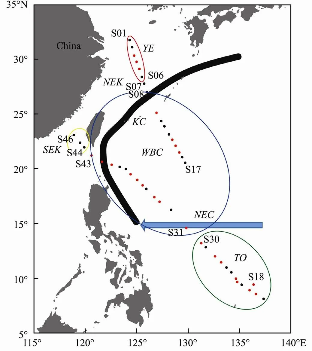
Fig.1 Locations of stations sampled in the western Pacific Ocean during winter 2014. Red symbols, daytime; Black symbols, nighttime; YE, Yangtze Delta-East China Sea water mass; NEK, northern East China Sea-Kuroshio Current water mass; SEK, southern East China Sea-Kuroshio Current water mass; WBC, Pacific western boundary current water mass; TO, tropical ocean. The approximate position of Pacific western boundary currents is depicted: KC, Kuroshio Current; NEC, North Equatorial Current (Hu et al., 2015).

2.2 Sampling Analysis

2.2.1 Analysis of environmental variables

Nutrients were analyzed with a SEAL QuAAtro auto- analyzer (SEAL Analytical Incorporation, Germany). The naphthylenediamine method, the cadmium reduction method, the indophenol blue method, the molybdenum- antimony-ascorbic method and the silicone molybdenum blue method were used for nitrate, nitrite, ammonium, phosphate and silicate analysis, respectively. The availability of dissolved inorganic nitrogen (DIN) is estimated as the sum of the concentrations of nitrate, nitrite and ammonium.

Chlorophyll(Chl-) was extracted using 90% acetone at −20℃ in the dark for 24h. Chl-concentrations were determined using a Turner Design (Model II) fluorometer, which was calibrated using pure chlorophyll (Sigma) (Jeffrey and Humphrey, 1975).

2.2.2 Analysis of zooplankton sample

Each zooplankton sample was divided into 3 subsamples by filtering through sieves with 300 and 100μm mesh sizes. Zooplankton < 100μm and 100–300μm were analyzed using a FlowCAM (Fluid Imaging Technologies Incorporation, USA), which scanned through the flow cell using a 4× objective lens. After processing the samples using the FlowCAM, detected objects were automatically classified, according to the library of plankton, followed by manual correction (Romero-Martinez., 2017). The zooplankton >300μm were scanned in the scanning cell (11×24cm2) of a semi-automatic ZooScan system (Hydroptic Incorporation, France) and digitized at a resolution of 4800 dpi. After processing with ZooProcess, detected objects were classified automatically, according to a learning set, followed by manual corrections (Schul- tes and Lopes, 2009; Gorsky., 2010). The samples were identified into the taxa, including Amphipoda, Chaetognatha, Copepoda, Euphausiacea, larvae, Medusa, nauplius, Polychaeta, Tunicata and other zooplankton and were counted according to the taxa.

The biovolume of zooplankton taxa is calculated from the equivalent spherical diameter (ESD) data. ESD values (mm) are converted to biovolume using the following formula:

The abundance per cubic meter (: indm−3) and the volume per cubic meter (: mm3m−3) for each of zooplankton taxa are calculated with the following equation:

whereis the number of particles (= zooplankton ind) or the volume of particles (= zooplankton mm3) andis the filtered volume of the net (m3).

2.3 Normalized Biovolume Size Spectra (NBSS)

According to the FlowCAM data and ZooScan data, the NBSS () is calculated (Platt and Denman, 1977):

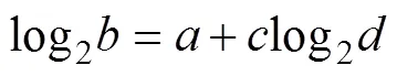
whereis the body volume of the zooplankton body in mm3. To compare biovolume spectra in different regions, the slope of the biovolume spectrum on the logarithm coordinates with base 2 is computed by using the least- squares fit of a linear function (Kerr and Dickie, 2001):

whereis the intercept of regression;is the slope of regression andis zooplankton biovolume (mm3m−3) in the abundance of each size class (indm−3). NBSS parameters such as the intercept and slope values are used to describe plankton community properties (Zhou, 2006). A higher intercept value indicates a higher organism abundance and vice versa (Kerr and Dickie, 2001; Jennings and Brander, 2010).

2.4 Statistical Analysis

Statistical analysis was performed using IBM SPSS 20.0 and R 3.5.2 (R Development Core Team, 2018). All data were normalized to mean and variance values of zero and one, respectively, to reduce the influence of the variance. Cluster analysis was performed to evaluate spatial variation based on hydrographic conditions (Johnson, 1967). Non-metric multidimensional scaling (NMDS) analyses were conducted to determine the environmental heterogeneity of zooplankton communities (Kruskal, 1964; Darnis., 2008). Shepard plots with low scatter suggest original dissimilarities are well preserved in the reduced number of dimensions (De Leeuw, 2017).Permutational multivariate analysis of variance (PERMANO VA) was conducted to test the differences in the zooplankton taxa among the water masses and between daytime and nighttime in the water mass (Michal., 2015; Anderson, 2017). To clarify how hydrographic conditions and environmental variables were related to the characteristic of zooplankton communities from inshore waters to the open ocean in the western Pacific Ocean, multiple linear regression (MLR) analysis and redundancy analysis (RDA) were performed (Färber-Lorda., 2004; Gao., 2008; Wang., 2018). MLR attempts to model the relationship between two or more explanatory variables and a response variable by fitting a linear equation to observed data, as follows:

whereis the value for the parameters of the plankton community structure, andXis the value for each corresponding environmental variable (Kutner and Nachts, 2005). Models are implemented in R and are stepwise using the Akaike information criterion (AIC) to identify the optimal explanatory variables. Finally, by means of the-value, the significance of the relationships between the explanatory variables and the response variable is evaluated(Kutner and Nachts, 2005).

3 Results

3.1 Hydrographic Conditions and Environmental Variables

Based on the hydrographic conditions, the western Pacific Ocean was classified into subtropical ocean and tropical ocean (TO) (Fig.2). The subtropical ocean included Yangtze Delta-East China Sea water mass (YE) located at the northern inshore waters, the East China Sea-Kuroshio Current water mass (EK) located at the boundary of the inshore waters and the open ocean, with a northern water mass (NEK) and a southern water mass (SEK), and Pacific western boundary currents water mass (WBC).

Fig.2 Dendrogram for stations based on Ward’s method using hydrographic condition data.

Fig.3 Spatial distribution of temperature and salinity in western Pacific Ocean during the winter of 2014.

The sea surface temperature (SST) ranged from 17.6 to 29.1℃ and exhibited a tendency to increase from inshore waters to the open ocean (Fig.3). The highest SST occurred at the tropical ocean, and SST slightly decreased to the north until the Kuroshio Current, where SST suddenly dropped to the north (Fig.3 and Table 1). The sea surface salinity (SSS) ranged from 33.72 to 34.79 psu (Fig.3). In the inshore waters, SST and SSS were positively correlated (=0.007<0.01). However, in the open ocean, SST and SSS were negatively correlated (= 0.000<0.01).

The sea surface Chl-ranged from 0.003 (open ocean) to 0.393 (inshore waters) μgL−1(Fig.4). The concentrations of sea surface DIN, PO43−-P, and SiO32−-Si ranged from 0.904 (open ocean) to 16.977 (inshore waters) μmolL−1, 0.014 (open ocean) to 1.593 (inshore waters) μmolL−1and 0.566 (open ocean) to 17.055 (inshore waters) μmolL−1, respectively (Fig.4). Environmental variables showed a spatial pattern opposite to that of SST and thus were higher in the inshore waters (YE and EK) and lowest in the open ocean (WBC and TO) (Table 1). According to the nutrient ratios (Redfield, 1960; Justić, 1995), phosphorus limitation existed in most of the surveyed areas except for in NEK and silicon limitation existed in the open ocean (Table 1 and Fig.5).

Table 1 Hydrographic conditions and environmental variables in the western Pacific Ocean during the winter of 2014

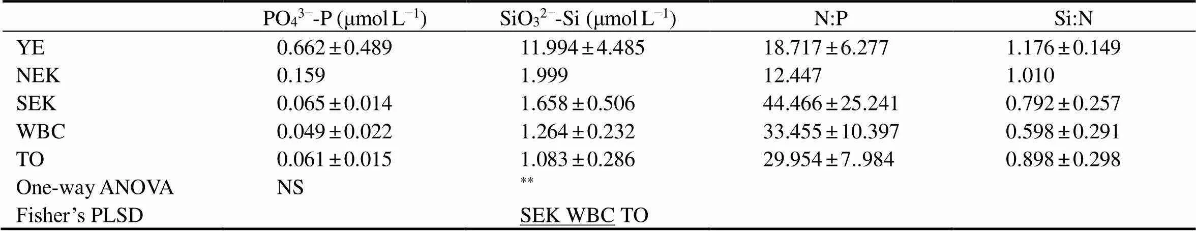
PO43−-P (μmolL−1)SiO32−-Si (μmolL−1)N:PSi:N YE0.662±0.48911.994±4.48518.717±6.2771.176±0.149 NEK0.1591.99912.4471.010 SEK0.065±0.0141.658±0.50644.466±25.2410.792±0.257 WBC0.049±0.0221.264±0.23233.455±10.3970.598±0.291 TO0.061±0.0151.083±0.28629.954±7..9840.898±0.298 One-way ANOVANS** Fisher’s PLSDSEK WBC TO

Notes: Values are mean ± standard deviation. Differences between the SEK, WBC and TO were tested by one-way ANOVA and Fisher’s PLSD. Any two zones not connected by underlines are significantly different (Fisher’s PLSD,*< 0.05,**< 0.01; NS, not significant).

Fig.4 Spatial distribution of Chl-a and nutrients in the western Pacific Ocean during the winter of 2014.

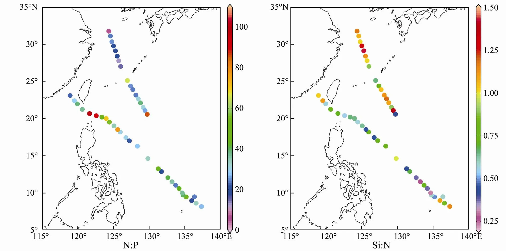
Fig.5 Spatial distribution of the N:P ratio and Si:N ratio in the Western Pacific Ocean during the winter of 2014.

3.2 Abundance and Biovolume of Zooplankton

The abundance and biovolume of zooplankton ranged from 40.0 to 15119.5indm−3and 33.26 to 9069.43mm3m−3, respectively (Fig.6). In general, abundance and biovolume decreased from the inshore waters towards the open ocean, showing a spatial pattern opposite to that of SST.

Fig.6 Spatial distribution of zooplankton abundance and biovolume in the western Pacific Ocean during the winter of 2014.

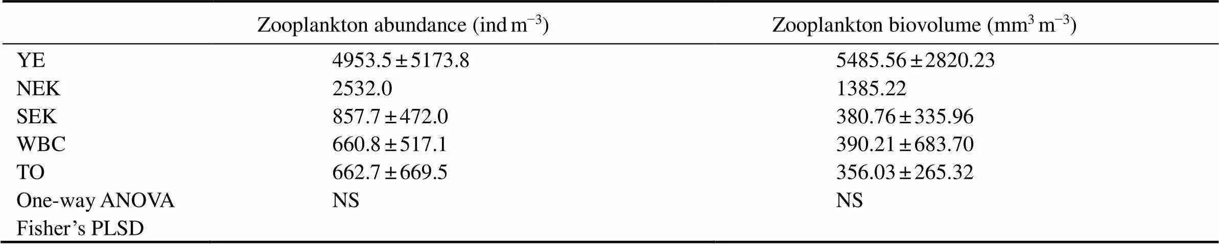
Table 2 Zooplankton abundance and biovolume in the western Pacific Ocean during the winter of 2014

Notes: Values are mean ± standard deviation. Differences between the SEK, WBC and TO were tested by one-way ANOVA and Fisher’s PLSD. Any two zones not connected by underlines are significantly different (Fisher’s PLSD,*< 0.05,**< 0.01; NS, not significant).

3.3 Zooplankton Community Composition

The zooplankton community compositions in the five water masses are shown in Fig.7. Chaetognatha, Copepoda, Euphausiacea, Medusa and nauplius were dominant zooplankton taxa from inshore waters to the open ocean. Copepoda wasthe dominant taxon and constituted 49.9% of the total biovolume from inshore waters to the open ocean. The proportion of Copepoda was lower in the inshore waters than in the open ocean. Copepoda constituted 36.0%, 47.3%, 50.4%, 50.1% and 56.1% of the total biovolume in YE, NEK, SEK, WBC and TO, respectively. In addition, NMDS analysis of zooplankton taxa among water masses indicated two distinct zooplankton assemblages (Fig.8). Euphausiacea was the second most dominant zooplankton taxon in some water masses; for example, it constituted 49.8% and 40.3% of the total biovolume in YE and NEK, respectively (Fig.7). Gelatinous zooplankton are generally considered to include Medusa and Tunicata (Alldredge, 1984). In SEK, WBC and TO, gelatinous zooplankton constituted 21.71%, 19.42% and 17.82% of the total biovolume, respectively (Fig.7). At the S01 station, gelatinous zooplankton constituted 9.30% of the total biovolume and in the SEK, and Chaetognatha constituted 18.73% of the total biovolume (Fig.7).

Zooplankton taxa composition based on the biovolume showed significant differences between YE and other water masses (YE and SEK, F=6.67,=0.009 <0.01; YE and WBC, F=11.25,=0.001 <0.01; YE and TO, F=13.37,=0.001<0.01). However, zooplankton taxa com- position based on the biovolume showed no significant difference between WBC and TO (F=0.95,= 0.422 >0.05). In addition, diurnal changes in zooplankton community structure showed no significant difference within the water masses (YE, F=2.86,=0.100 >0.05; WBC, F=0.88,=0.46 > 0.05; TO, F=0.56,=0.791> 0.05).

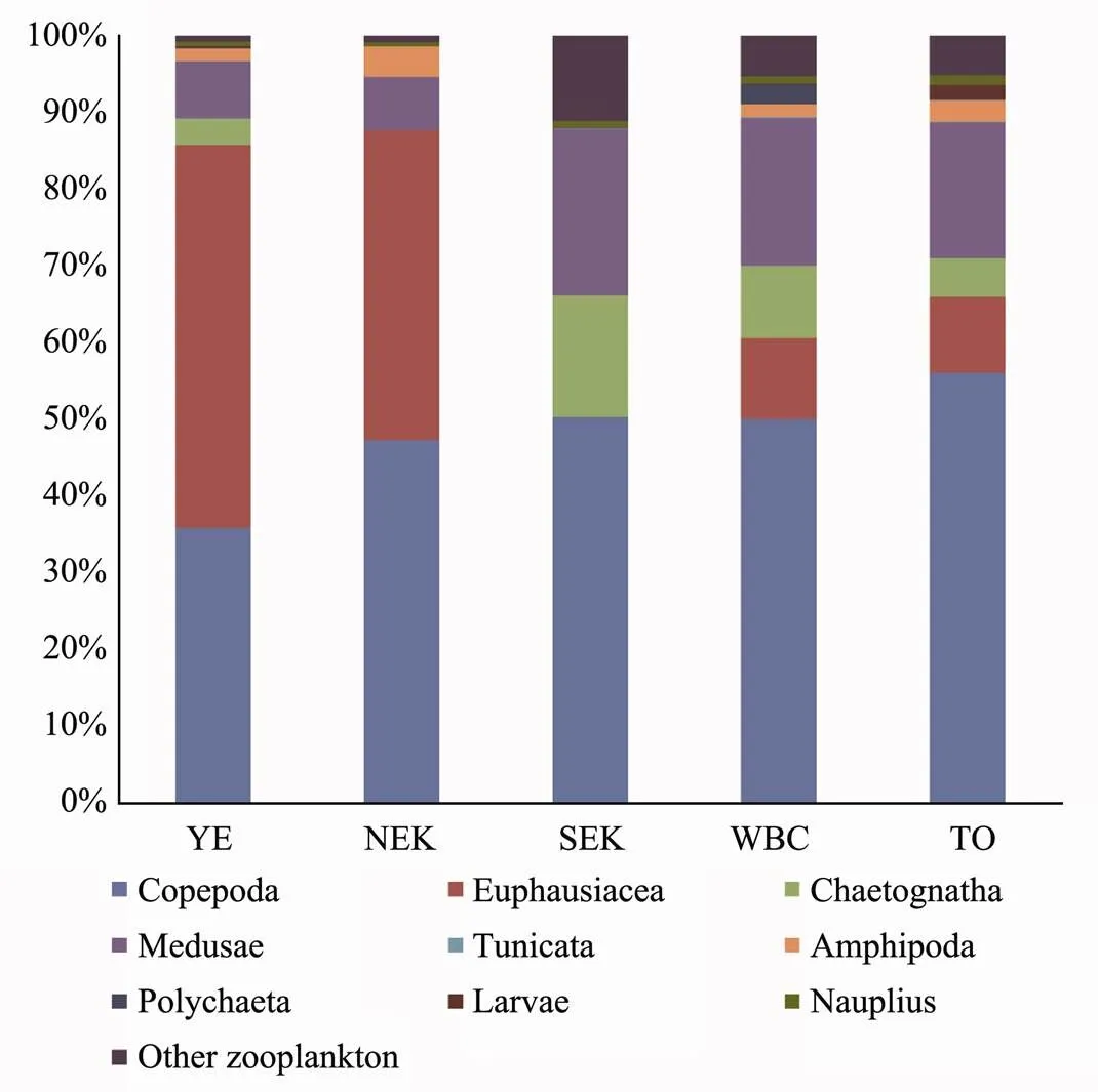
Fig.7 Zooplankton taxa composition in the western Pacific Ocean during winter 2014.

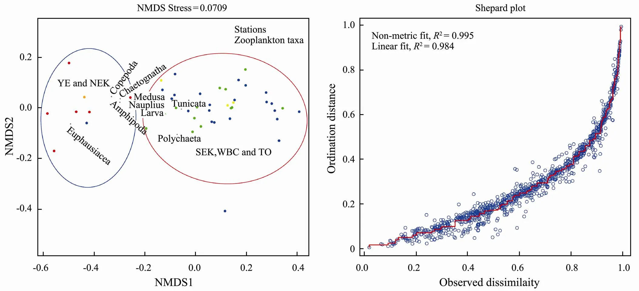
Fig.8 NMDS analysis of the zooplankton taxa and water masses and Shepard plot. Red solid circle, YE; orange solid circle, NEK; yellow solid circle, SEK; blue solid circle, WBC; green solid circle, TO.

In addition, zooplankton taxa composition based on the total abundance of each size class showed significant differences among water masses during winter 2014 from inshore waters to the open ocean (Fig.9). In the 0.077–1 mm ESD size class, Copepoda and nauplius dominated, accounting for >90% of zooplankton abundance, and the proportion of Copepoda was lower in YE and NEK than in SEK, WBC and TO. Copepoda also dominated the 1–2, 2–3 and 3–4 mm ESD size classes.In the northern inshore waters (YE and NEK), the proportion of Copepoda in the zooplankton abundance decreased as the size classes increased, whereas that of Euphausiacea increased. In SEK, the proportion of Copepoda in the zooplankton abundance decreased as the size classes increased, whe- reas that of gelatinous zooplankton and Chaetognatha increased. In WBC, the proportion of Copepoda in the zooplankton abundance decreased as the size class increased, whereas that of gelatinous zooplankton, Chaetognatha and Euphausiacea increased. In TO, the proportion of Copepoda in the zooplankton abundance decreased as the size class increased, whereas that of gelatinous zooplankton and Euphausiacea increased.

Fig.9 Abundance composition of zooplankton taxa in each size class in the western Pacific Ocean during the winter of 2014.

3.4 NBSS of Zooplankton

Fig.10 shows the slopes and intercepts of NBSS from inshore waters to the open ocean. The slopes of the NBSS ranged from −0.56 to −1.36 and no significant differences among water masses were observed (as shown in Table3). Steeper NBSS slopes were found in the Yangtze River Delta and SEK (Fig.10 and Table3). The intercepts of the NBSS ranged from 0.44 to 6.10. The average intercepts in five water masses were ranked as following: NEK (5.90) > YE (4.87) > TO (2.73) > SEK (2.27) > WBC (1.96).

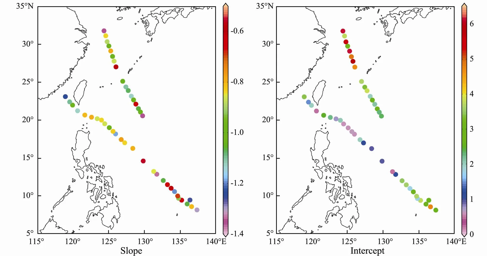
Fig.10 Spatial distribution of the slope and intercept of the NBSS in the western Pacific Ocean during the winter of 2014.

Table 3 The slope and intercept of NBSS in the western Pacific Ocean during the winter of 2014

Notes: Values are mean ± standard deviation. Differences between the YE, NEK, SEK, WBC and TO were tested by one-way ANOVA and Fisher’s PLSD. Any two zones not connected by underlines are significantly different (Fisher’s PLSD,*< 0.05,**< 0.01; NS, not significant).

3.5 The Relationship Between Zooplankton Com- munities and Environmental Factors

The MLR and RDA results demonstrated that environmental variables did affect the abundance and biovolume of zooplankton and the spatial distribution of zooplankton taxa from inshore waters to the open ocean (Table 4, Table 5 and Fig.11). With the greater availability of nutrients and Chl-in the inshore waters, more zooplankton were sustained than in the open ocean andzooplankton biomass was lower under conditions of higher SST and SSS in the open ocean (Table 4). However, in the inshore waters, zooplankton biovolume was negatively related to Chl-and DIN (Table 4). In addition, the MLR results demonstrated that the NBSS slope was negatively related to Chl-and PO43−-P in the inshore waters, while in the open ocean (WBC and TO), the NBSS slope, did not demonstrate any relationship with environmental conditions.

Table 4 Results of the MLA models obtained from exploring the relationships between zooplankton abundance, zooplankton biovolume, slope and SST, SSS, Chl-a, DIN, PO43−-P and SiO32−-Si

Notes:*means significance;**means extreme significance.-values are shown just as reference as these dependent variables are influenced by the number of explanatory variables.

Table 5 Monte Carlo permutation test of the RDA models determined by forward stepwise selection of hydrography conditions and environmental variables explaining the distribution of zooplankton communities

Notes:*means significance;**means extreme significance.

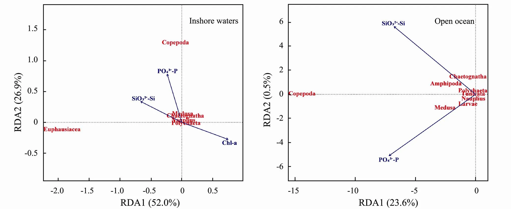
Fig.11 RDA plot of zooplankton communities and hydrographic conditions and environmental variables in the western Pacific Ocean during the winter of 2014.

4 Discussion

4.1 Abundance and Biovolume

We investigated spatial distribution of zooplankton abundance and biovolume at large scale from inshore waters to the open ocean in the western Pacific Ocean during the winter of 2014. We found that the characteristics (hydrographic conditions and environmental variables) of water mass largely explained the spatial variation in zooplankton abundance and biovolume (Table 4). Thestudy area was under strong influence of Pacific western boundary currents and was subdivided into continental margins and the deep ocean; thus, the hydrographic conditions and environmental variables were completely different from inshore waters to the open ocean. In the inshore waters, the water mass of the East China Sea mid- shelf region comprises largely of Yangtze River diluted water and oceanic Kuroshio Water (Chen., 1995; Ichikawa and Beardsley, 2002; Chen., 2008). Yangtze River diluted water is rich in nitrogen nutrients(Müller., 2008; Gao., 2012). It is usually the dominant water mass, so YE is considered to be phosphate limited (Table 1). Hirst and Bunker (2003) pointed out that under food-limited conditions, the biomass of Copepoda may be heavily dependent on the availability of the limiting resource. Some research in the fields also indicated that the growth and fecundity of zooplankton mainly depend on the limited resource (Hopcroft., 1998; Zhou., 2018). Indeed, our results demonstrated that zooplankton abundance was positively related to PO43−-P in the inshore waters (Table 4). In the oligotrophic ocean area, the characteristic of water masses (WBC and TO) showed the difference in temperature, salinity and SiO32−-Si (Table 1). Physical oceanography processes, such as the current and the equatorial upwelling, could significantly influence the distribution patterns of zooplankton biomass (Roman., 2002; Fernández-Álamo and Färber-Lorda, 2006; Salas-de-León., 2011). Based on our clusters, in the open ocean, WBC was mainly influenced by Pacific western boundary currents with a feather of higher SST and lower PO43−-P concentrations and TO was mainly influenced by the equatorial tropical zone in the Pacific Ocean with a feather of higher SSS, lower SST and lower SiO32−-Si concentrations (Table 1). According to Liebig’s law of the minimum-growth controlled not by the total amount of resources availablebut by the scarcest resource, the characteristics of the water mass were coupled with the zooplankton abundance and biovolume in response to hydrographic conditions and environmental variables in the open ocean (Table 4). Previous studies also suggested that spatial variation in zooplankton communities was in accordance with water mass (the Yellow Sea cold water mass, the Yangtze River diluted water and currents) in the western Pacific Ocean (Wu., 2000; Qiu., 2010; Dai., 2016; Fan., 2016). Taken together, we infer that zooplankton abundance and biovolume may possibly be affected by limited and scarce nutrients in the water mass from inshore waters to the open ocean in the western Pacific Ocean during the winter of 2014.

We also found that areas with higher Chl-concentrations tended to have lower zooplankton biovolume in the inshore waters during the winter of 2014 (Table 4). This result, however, was opposite to what is predicted by theoretical models. Theoretical models predict an increasing biomass of zooplankton with increased food availability (Froneman, 2001; Finenko., 2003). A possible reason for this contradictory finding may be that the biomass of zooplankton was possibly controlled by the dominant zooplankton taxa (Purcell., 1994; Schneider and Behrends, 1998). Previous studies also suggested that as the herbivores in the zooplankton community, Euphausiacea can be more efficient in consuming primary producer as high as 50% (Holm-Hansen and Huntley, 1984; Perissinotto, 1997), which leads to a higher biomass of zooplankton. However, herbivores were less efficient in using primary production when they were constrained by omnivores and carnivorous, which led to a lower biomass of zooplankton (Purcell., 1994; Pagès., 1996). Indeed, a higher proportion of Euphausiacea and gelatinous zooplankton occurred in the northern inshore waters (YE and NEK) and SEK as the dominant zooplankton taxa, respectively (Fig.7 and Fig.9), which might have led to a different response of the zooplankton biomass to primary production (Chl-). Overall, our observations suggested that a negative relationship between zooplankton biovolume and Chl-concentration occurred in the inshore waters during the winter of 2014, perhaps due to the difference in dominant zooplankton taxa.

4.2 Spatial Variation in Zooplankton Community Structure

Based on the results described above, a significant spatial variation in zooplankton community structure was confirmed among the water masses in the western Pacific Oceanduring the winter of 2014. The proportion of Copepoda showed more variation among the water masses from inshore waters to the open ocean (Fig.7). The difference in the proportion of Copepoda between the northern inshore waters (YE and NEK) and SEK may be related to the dominant zooplankton taxa. Euphausiacea as herbivores was more efficient in using primary production, compared with Chaetognatha and gelatinous zooplankton as carnivores (Purcell., 1994; Schneider and Behrends, 1998; Terazaki, 2000). In addition, it has been reported that the slopes of the NBSS can be influenced by top-down effects. Top-down processes such as predation by carnivores species that selectively feed on zooplankton in larger size classes also lead to steeper slopes (Moore and Suthers, 2006). Indeed, the steepest slope of the NBSS in SEK may be due to the higher abundance proportion of smaller size classes, higher proportion of Chaetognatha and gelatinous zooplankton in total biovolume (Fig.7) and higher proportion of nauplius in the 0.077 to 1mm ESD size (Fig.9) class than in the northern inshore waters. Overall, our observations suggested that spatial variation in zooplankton community structure in the inshore waters was primarily due to the top-down effects of dominant zooplankton taxa.

In addition, after Copepoda, Euphausiacea was the dominant zooplankton taxon in the northern inshore waters (YE and NEK), and gelatinous zooplankton was the second most dominant zooplankton taxon in the open ocean (Fig.7 and Fig.9). The difference in the zooplankton community composition between the northern inshore waters and in the open ocean may be related to the characteristics of the water masses. In the inshore waters, under conditions of sufficient food resource, the proportion of large predators is expected to be balanced and maximized in the marine ecosystem (López-López., 2013). In our study, Copepoda prefered higher PO43−-P concentrations and Euphausiacea prefered higher SiO3-Si concentrations (Fig.11). Food resources are considered one of the most important factors influencing the distribution of Euphausiacea. Assemblages with abundant Euphausiacea have been reported in cooler and nutrient-rich water (Yoon., 2000). Hence, a high biovolume of Euphausiacea was detected in the northern inshore as the dominant zooplankton taxon. However, in the open ocean, a low-energy food chain favors nanoplankton and Medusa (Parsons and Lalli, 2002). Copepoda had a higher biovolume proportion, mainly due to the greater contribution of the small body-size individuals in the open ocean (Agawin., 2000; Mackinson., 2015). In addition, hydrographic conditions are considered one of the most important factors influencing the distribution of gelatinous zooplankton (Bieri, 1959; Pagès and Gili, 1991; Ulloa., 2000). Assemblages with abundant gelatinous zooplankton have been reported in warmer waters (Graham., 2001). In the current study, the proportion of gelatinous zooplankton was higher in the open ocean where SST and SSS were high. Besides, we found that Medusa were positively associated with SiO32−-Si (Fig.11). In the open ocean, under the generally stable temperature and light conditions, the plankton community can respond rapidly to nutrient enhancement (Furnas., 2005). Thus, gelatinous zooplankton as the dominant zooplankton taxon in the open ocean responded to increased productivitythe food chain. Accordingly, a high proportion of gelatinous zooplankton was found in the open ocean during the winter of 2014.

4.3 NBSS of Zooplankton

Our results agreed with a positive relationship between environmental variables (Chl-and PO43−-P) and NBSS steepness in the inshore waters during the winter of 2014 (Table 4). Stations with steeper NBSS slopes corresponded to areas of high Chl-concentrations and PO43−- P concentrations. Thus,steeper NBSS slopeswere usually present in the YE (S01) and SEK. The slope of the NBSS is determined by the energy transfer efficiency and number of trophic levels and is an inherent property of a community (Zhou, 2006). In general, steeper NBSS slopes mean the increase in the food limitation to larger size classes (Zhou, 2006). However, our results may suggest another process. Following the metabolic theory of ecology, the slope of NBSS is −0.75 within trophic level and −1 across all trophic levels (Brown and Gillooly, 2003, Brown., 2004). The slope, with the value −1.17 in t YE (S01) and SEK, was closer the estimate of −1 across all trophic levels than the estimate of −0.75 within a trophic level. Based on the NBSS slope value and zooplankton community trophic level (Zhou, 2006), the trophic level of the zooplankton community in YE (S01) and SEK was 2.72, while that in the other areas was 2.12. This indicated that a higher proportion of carnivore zooplankton occurred in YE (S01) and SEK. In our study, Chaetognatha and gelatinous zooplankton as carnivores were the dominant zooplankton taxa in YE (S01) and SEK (Fig.7), which might lead more trophic levels with the longer food chain. In addition, energy transfer efficiency from low trophic levels to high trophic levels is higher in shorter food chains(Dickman., 2008). Therefore, the positive relationship between environmental variables (Chl-and PO43−-P) and NBSS steepness showed the energy transfer efficiency of zooplankton communitiesin response to the dominant zooplankton taxa in the inshore waters during the winter of 2014 and more importantly, higher trophic levels induced the stee- per NBSS slopes

5 Conclusions

Based on the spatial variation in zooplankton community characteristics and its relationship with the environmental factors in the western Pacific Ocean, our results indicated that the effect of environmental characteristic (limited and scarcer nutrients) as main control factors of water mass on the zooplankton abundance and biovolume from inshore waters to the open ocean.It was found that the spatial distribution of zooplankton taxa among the water masses could mainly depend on i) the difference in the environmental conditions between the inshore waters and the open ocean and ii) the top-down effects of the dominant zooplankton taxa in the inshore waters. Moreover, the negative relationship between zooplankton biovolume and Chl-concentrations represented a meaningful pattern, which may be due to the difference in dominant zooplankton taxa. A higher trophic level of the dominant zooplankton taxa resulted in a steeper NBSS slope in the inshore waters. Temporal variability of zooplankton communities and the ecological distribution of zooplankton in this region are still poorly known, and further studies of zooplankton in this region should be conducted.

Acknowledgements

This work was supported by the Key Research Program of Frontier Sciences of the Chinese Academy of Sciences (No. QYZDB-SSW-DQC02402), the Strategic Priority Research Program of the Chinese Academy of Sciences (No. XDB42030402), the Science & Technology Basic Resources Investigation Program of China (No. 2017FY100803), the International Science Partnership Program of the Chinese Academy of Sciences (No. 133 137KYSB20200002), and the National Natural Science Foundation of China (No. 91751202). We are grateful to the captain and crew of‘’ for their technical and logistical support.

Agawin, N. S. R., Duarte, C. M., and Agustí, S., 2000. Nutrient and temperature control of the contribution of picoplankton to phytoplankton biomass and production., 45 (3): 591-600, DOI: 10.4319/lo.2000.45.3. 0591.

Alldredge, A. L., 1984. The quantitative significance of gelatinous zooplankton as pelagic consumers. In:. Fasham, M. J. R., and Boston, MA, Springer US,407-433.

Anderson, M. J., 2017. Permutational multivariate analysis of variance (PERMANOVA)., 1-15.

Badosa, A., Boix, D., Brucet, S., López-Flores, R., Gascón S., and Quintana, X. D., 2007. Zooplankton taxonomic and size diversity in Mediterranean coastal lagoons (NE Iberian Peninsula): Influence of hydrology, nutrient composition, food resource availability and predation., 71 (1): 335-346, DOI: 10.1016/j.ecss.2006.08. 005.

Bieri, R., 1959. The distribution of the planktonic Chaetognatha in the Pacific and their relationship to the water masses., 4 (1): 1-28, DOI: 10.4319/lo. 1959.4.1.0001.

Boucher, J., Ibanez, F., and Prieur, L., 1987. Daily and seasonal variations in the spatial distribution of zooplankton populations in relation to the physical structure in the Ligurian Sea Front., 45 (1): 133-173, DOI: 10. 1357/002224087788400891.

Brown, J. H., and Gillooly, J. F., 2003. Ecological food webs: High-quality data facilitate theoretical unification., 100 (4): 1467-1468, DOI: 10.1073/pnas.0630310100.

Brown, J. H., Gillooly, J. F., Allen, A. P., Savage, V. M., and West, G. B., 2004. Toward a metabolic theory ecology., 85 (7): 1771-1789, DOI: 10.1890/03-9000.

Candu, C., and Saleur, H., 2010. Geographical shift of zooplankton communities and decadal dynamics of Kuroshio- Oyashio currents in the western North Pacific., 15 (7): 1846-1858, DOI: 10.1111/j.1365- 2486.2009.01890.x.

Chen, C., Xue, P., Ding, P., Beardsley, R. C., Xu, Q., Mao, X., Gao, G., Qi, J., Li, C., Lin, H., Cowles, G., and Shi, M., 2008. Physical mechanisms for the offshore detachment of the Changjiang diluted water in the East China Sea., 113 (C2): C02002, DOI: 10. 1029/2006JC003994.

Chen, C. T. A., Ruo, R., Paid, S. C., Liu, C. T., and Wong, G. T. F., 1995. Exchange of water masses between the East China Sea and the Kuroshio off northeastern Taiwan., 15 (1): 19-39, DOI: 10.1016/0278-4343(93) E0001-O.

Dai, L., Li, C., Yang, G., and Sun, X., 2016. Zooplankton abundance, biovolume and size spectra at western boundary currents in the subtropical North Pacific during winter 2012., 155: 73-83, DOI: 10.1016/j. jmarsys.2015.11.004.

Darnis, G., Barber, D. G., and Fortier, L., 2008. Sea ice and the onshore-offshore gradient in pre-winter zooplankton assemblages in southeastern Beaufort Sea., 74 (3-4): 994-1011, DOI: 10.1016/j.jmarsys.2007.09. 003.

Dickman, E. M., Newell, J. M., González, M. J., and Vanni, M. J., 2008. Light, nutrients, and food-chain length constrain planktonic energy transfer efficiency across multiple trophic levels., 105 (47): 18408-18412, DOI: 10.1073/pnas.0805566105.

Dvoretsky, V. G., and Dvoretsky, A. G., 2015. Regional differences of mesozooplankton communities in the Kara Sea., 105: 26-41, DOI: 10.1016/j.csr. 2015.06.004.

Fan, R., Wei, H., and Zhao, L., 2016. Linking suspended particulate material characteristics to the plankton distribution in summer in the Yellow Sea and East China Sea., 32 (4): 829-839, DOI: 10.2112/JCOAST RES-D-15-00094.1.

Färber-Lorda, J., Trasviña, A., and Verdı́n, P. C., 2004. Trophic conditions and zooplankton distribution in the entrance of the Sea of Cortés during summer., 51: 615-627, DOI: 10. 1016/j.dsr2.2004. 05.003.

Fernández-Álamo, M. A. and Färber-Lorda, J., 2006. Zooplankton and the oceanography of the eastern tropical Pacific: A review., 69 (2): 318-359, DOI: 10. 1016/j.pocean.2006.03.003.

Finenko, Z. Z., Piontkovski, S. A., Williams, R., and Mishonov, A. V., 2003. Variability of phytoplankton and mesozooplankton biomass in the subtropical and tropical Atlantic Ocean., 250: 125-144, DOI: 10.33 54/meps250125.

Frederiksen, M., Edwards, M., Richardson, A. J., Halliday, N. C., and Wanless, S., 2006. From plankton to top predators: Bottom-up control of a marine food web across four trophic levels., 75 (6): 1259-1268, DOI: 10. 1111/j.1365-2656.2006.01148.x.

Froneman, P. W., 2001. Seasonal changes in zooplankton biomass and grazing in a temperate estuary, South Africa., 52 (5): 543-553, DOI: 10. 1006/ecss.2001.0776.

Fuchs, H., and Franks, P., 2010. Plankton community properties determined by nutrients and size-selective feeding., 413 (6): 1-15, DOI: 10.3354/meps08716.

Furnas, M., Mitchell, A., Skuza, M., and Brodie, J., 2005. In the other 90%: Phytoplankton responses to enhanced nutrient availability in the Great Barrier Reef Lagoon., 51 (1): 253-265, DOI: 10.1016/j.marpolbul. 2004.11.010.

Gao, L., Li, D., and Zhang, Y., 2012. Nutrients and particulate organic matter discharged by the Changjiang (Yangtze River): Seasonal variations and temporal trends., 117: G04001, DOI: 10. 1029/2012JG001952.

Gao, Q., Xu, Z., and Zhuang, P., 2008. The relation between distribution of zooplankton and salinity in the Changjiang Estuary., 26 (2): 178-185, DOI: 10.1007/s00343-008-0178-1.

Gorsky, G., Ohman, M. D., Picheral, M., Gasparini, S., Stemmann, L., Romagnan, J. B., Cawood, A., Pesant, S., Garcia-Comas, C., and Prejger, F., 2010. Digital zooplankton image analysis using the ZooScan integrated system., 32 (3): 285-303, DOI: 10.1093/plankt/ fbp124.

Graham, W. M., Pagès, F., and Hamner, W. M., 2001. A physical context for gelatinous zooplankton aggregations: A review., 451 (1): 199-212, DOI: 10.1023/A:1011876 004427.

Hayward, T. L., Venrick, E. L., and Mcgowan, J. A., 1983. Environmental heterogeneity and plankton community structure in the central North Pacific., 41 (4): 711-729, DOI: 10.1357/002224083788520441.

Helenius, L. K., Leskinen, E., Lehtonen, H., and Nurminen, L., 2016. Spatial patterns of littoral zooplankton assemblages along a salinity gradient in a brackish sea: A functional diversity perspective., 198: 400-412, DOI: 10.1016/j.ecss.2016.08.031.

Hirst, A. G., and Bunker, A. J., 2003. Growth of marine planktonic copepods: Global rates and patterns in relation to chlorophyll, temperature, and body weight., 48 (5): 1988-2010, DOI: 10.4319/lo.2003.48. 5.1988.

Holm-Hansen, O., and Huntley, M., 1984. Feeding requirements of krill in relation to food sources., 4: 156-173, DOI: 10.1163/1937240X84X00 561.

Holste, L., John, M. A. S., and Peck, M. A., 2009. The effects of temperature and salinity on reproductive success ofin the Baltic Sea: A copepod coping with a tough situation., 156 (4): 527-540, DOI: 10.1007/ s00227-008-1101-1.

Hopcroft, R. R., Roff, J. C., Webber, M. K., and Witt, J. D. S., 1998. Zooplankton growth rates: The influence of size and resources in tropical marine copepodites., 132 (1): 67-77, DOI: 10.1007/s002270050372.

Hu, D., Wu, L., Cai, W., Gupta, A. S., Ganachaud, A., Qiu, B., Gordon, A. L., Lin, X., Chen, Z., Hu, S., Wang, G., Wang, Q., Sprintall, J., Qu, T., Kashino, Y., Wang, F., and Kessler, W. S., 2015. Pacific western boundary currents and their roles in climate., 522: 299-308, DOI: 10.1038/nature14504.

Ichikawa, H., and Beardsley, R. C., 2002. The current system in the Yellow and East China Seas., 58 (1): 77-92, DOI: 10.1023/A:1015876701363.

Jeffrey, S. W., and Humphrey, G. F., 1975. New spectrophotometric equations for determining chlorophylls,,1 and2 in higher plants, algae and natural phytoplankton., 167 (2): 191-194, DOI: 10.1016/S0015-3796(17)30778-3.

Jennings, S., and Brander, K., 2010. Predicting the effects of climate change on marine communities and the consequences for fisheries., 79 (3): 418-426, DOI: 10.1016/j.jmarsys.2008.12.016.

Johnson, S. C., 1967. Hierarchical clustering schemes., 32 (3): 241-254, DOI: 10.1007/BF02289588.

Kerr, S. R., and Dickie, L. M., 2001.. Columbia University Press, New York, 1-22.

Kiørboe, T., 1997. Population regulation and role of mesozooplankton in shaping marine pelagic food webs., 363 (1): 13-27, DOI: 10.1023/A:1003173721751.

Krause, M., Dippner, J. W., and Beil, J., 1995. A review of hydrographic controls on the distribution of zooplankton biomass and species in the North Sea with particular reference to a survey conducted in January–March 1987., 35 (2): 81-152, DOI: 10.1016/0079-6611(95) 00006-3.

Kruskal, J., 1964. Nonmetric multidimensional scaling: A numerical method., 29 (2): 115-129, DOI: 10.10 07/BF02289694.

Kutner, M. H., and Nachts, C. J., 2005.. Higher Education Pressn; McGraw-Hill Education (Asia) Co.

Liu, P., Song, H., Wang, X., Wang, Z., Pu, X., and Zhu, M., 2012. Seasonal variability of the zooplankton community in the southwest of the Huanghai Sea (Yellow Sea) Cold Water Mass., 31 (4): 127-139, DOI: 10. 1007/sl3131-012-0226-8.

López-López, L., Molinero, J. C., Tseng, L. C., Chen, Q. C., and Hwang, J. S., 2013. Seasonal variability of the gelatinous carnivore zooplankton community in northern Taiwan., 35 (3): 677-683, DOI: 10.1093/plankt/ fbt005.

Mackas, D. L., Washburn, L., and Smith, S. L., 1991. Zooplank- ton community pattern associated with a California Current cold filament., 96 (C8): 14781-14797, DOI: 10.1029/91jc01037.

Mackinson, B. L., Moran, S. B., Lomas, M. W., Stewart, G. M., and Kelly, R. P., 2015. Estimates of micro-, nano-, and picoplankton contributions to particle export in the northeast Pacific., 12 (11): 3429-3446, DOI: 10.5194/ bg-12-3429-2015.

Michal, S., Thomas, A., Davidson, S., Rosemberg, B., and Menezes, F., 2015. Zooplankton response to climate warming: A mesocosm experiment at contrasting temperatures and nutrient levels., 745: 185-203, DOI: 10.1007/ s10750-014-1985-3.

Moore, S. K., and Suthers, I. M., 2006. Evaluation and correction of subresolved particles by the optical plankton counter in three Australian estuaries with pristine to highly modified catchments., 111 (C5): C05S04, DOI: 10.1029/2005JC002920.

Müller, B., Berg, M., Yao, Z. P., Zhang, X. F., Wang, D., and Pfluger, A., 2008. How polluted is the Yangtze river? Water quality downstream from the Three Gorges Dam., 402 (2): 232-247, DOI: 10.1016/j. scitotenv.2008.04.049.

Otto, S. A., Rabea, F, D., Georgs, J. K., and Christian, M. L., 2014. Habitat heterogeneity determines climate impact on zooplankton community structure and dynamics., 9 (3): e90875, DOI: 10.1371/journal.pone.0090875.

Pagès, F., and Gili, J., 1991. Effects of large-scale advective processses on gelatinous zooplankton populations in the northern Benguela ecosystem., 75 (2-3): 205-215, DOI: 10.3354/meps075205.

Pagès, F., González, H., and González, S., 1996. Diet of the gelatinous zooplankton in Hardangerfjord (Norway) and potential predatory impact by Aglantha digitale (Trachymedusae)., 139: 69-77, DOI: 10. 3354/meps139069.

Parsons, T. R., and Lalli, C. M., 2002. Jellyfish population explosions: Revisiting a hypothesis of possible causes., 40: 111-121.

Perissinotto, R., Pakhomov, E. A., McQuaid, C. D., and Froneman, P. W., 1997.grazing rates and daily ration of Antarctic krillfeeding on phytoplankton at the Antarctic Polar Front and the Marginal Ice Zone., 160: 77-91, DOI: 10.3354/meps160 077.

Pinel-Alloul, P., 1995. Spatial heterogeneity as a multiscale characteristic of zooplankton community., 300-301 (1): 17-42, DOI: 10.1007/BF00024445.

Piontkovski, S. A., and Landry, M. R., 2003. Copepod species diversity and climate variability in the tropical Atlantic Ocean., 12 (4‐5): 352-359, DOI: 10.1046/j. 1365-2419.2003.00250.x.

Platt, T. and K. Denman, 1977. Organisation in the pelagic ecosystem., 30 (1-4): 575-581, DOI: 10.1007/BF02207862.

Purcell, J. E., White, J. R., and Roman, M. R., 1994. Predation by gelatinous zooplankton and resource limitation as potential controls ofcopepod populations in Chesapeake Bay., 39 (2): 263-278, DOI: 10. 4319/lo.1994.39.2.0263.

Qiu, D. J., Huang, L. M., Zhang, J. L., and Lin, S. J., 2010. Phytoplankton dynamics in and near the highly eutrophic Pearl River Estuary, South China Sea., 30 (2): 177-186, DOI: 10.1016/j.csr.2009.10.015.

R Core Team, 2018. R: A language and environment for statistical computing. R Foundation for Statistical Computing, Vienna, Austria.

Roman, M. R., Dam, H. G., Le Borgne, R., and Zhang, X., 2002. Latitudinal comparisons of equatorial Pacific zooplankton., 49 (13): 2695-2711, DOI: 10.1016/S0967-0645(02)00054-1.

Romero-Martinez, L., van Slooten, C., Nebot, E., Acevedo- Merino A., and Peperzak, L., 2017. Assessment of imaging-in-flow system (FlowCAM) for systematic ballast water management., 603-604: 550-561, DOI: 10.1016/j.scitotenv.2017.06.070.

Rothlisberg, P. C., 1979. Combined effects of temperature and salinity on the survival and growth of the larvae of(Decapoda: Pandalidae)., 54 (2): 125- 134, DOI: 10.1007/BF00386591.

Sabatès, A., Gili, J. M., and Pagès, F., 1989. Relationship between zooplankton distribution, geographic characteristics and hydrographic patterns off the Catalan coast (Western Mediterranean)., 103 (2): 153-159, DOI: 10. 1007/BF00543342.

Salas-de-León, D. A., Carbajal, N., Monreal-Gómez, M. A., and Gil-Zurita, A., 2011. Vorticity and mixing induced by the barotropic M2tidal current and zooplankton biomass distribution in the Gulf of California., 66 (2): 143-153, DOI: 10.1016/j.seares.2011.05.011.

Schneider, G., and Behrends, G., 1998. Top-down control in a neritic plankton system bymedusae – A summary., 48 (2): 71-82, DOI: 10.1080/00785236.1998. 10428677.

Schultes, S., and Lopes, R. M., 2009. Laser optical plankton counter and zooscan intercomparison in tropical and subtropical marine ecosystems., 7: 771-784, DOI: 10.4319/lom.2009.7.771.

Schüβler, U., and Kremling, K., 1993. A pumping system for underway sampling of dissolved and particulate trace elements in near-surface waters., 40 (2): 257-266, DOI: 10. 1016/0967-0637(93)90003-L.

Sun, S., Tao, Z., Li, C., and Liu, H., 2011. Spatial distribution and population structure ofin the Yellow Sea (2006-2007)., 33 (6): 873-889, DOI: 10.1093/plankt/fbq160.

Terazaki, M., 2000. Feeding of carnivorous zooplankton, chaetognaths in the Pacific. In:. Handa, N., Tanoue, E., and Hama, T., eds., Springer Netherlands, Dordrecht, 257-276.

Tseng, L. C., Souissi, S., Dahms, H. U., Chen, Q. C., and Hw- ang, J. S., 2008. Copepod communities related to water mass- es in the southwest East China Sea., 62 (2): 153-165, DOI: 10.1007/s10152-007-0101-8.

Ulloa, R., Palma, S., and Silva, N., 2000. Bathymetric distribution of chaetognaths and their association with water masses off the coast of Valparaı́so, Chile., 47 (11): 2009-2027, DOI: 10.1016/S0967-0637(00)00020-0.

Vargas, C. D., Audic, S., Henry, N., Decelle, J., Mahé, F., Logares, R., Lara, E., Berney, C., Bescot, N. L., and Probert, I., 2016. Eukaryotic plankton diversity in the sunlit ocean., 348: 29223618-29223625, DOI: 10.1126/science.1261 605.

Vizzini, S., and Mazzola, A., 2006. Sources and transfer of organic matter in food webs of a Mediterranean coastal environment: Evidence for spatial variability., 66 (3-4): 459-467, DOI: 10.1016/j.ecss. 2005.10.004.

Wang, W., Sun, S., Zhang, F., Sun, X., and Zhang, G., 2018. Zooplankton community structure, abundance and biovolume in Jiaozhou Bay and the adjacent coastal Yellow Sea during summers of 2005–2012: Relationships with increasing water temperature., 36 (5): 1655-1670, DOI: 10.1007/s00343-018-7099-4.

Wu, Y. L., Zhang, Y. S., and Zhou, C. X., 2000. Phytoplankton distribution and community structure in the East China Sea (ECS) continental shelf., 18 (1): 74-79, DOI: 10.1007/BF02842545.

Yoon, W. D., Cho, S. H., Lim, D., Yong, K. C., and Lee, Y., 2000. Spatial distribution of(Euphausiacea: Crustacea) in the Yellow Sea., 22 (5): 939-949, DOI: 10.1093/plankt/22.5.939.

Zervoudaki, S., Nielsen, T. G., and Carstensen, J., 2009. Seasonal succession and composition of the zooplankton community along an eutrophication and salinity gradient exemplified by Danish waters., 31 (12): 1475-1492, DOI: 10.1093/plankt/fbp084.

Zhang, W., Tang, D., Yang, B., Gao, S., Sun, J., Tao, Z., Sun, S., and Ning, X., 2009. Onshore-offshore variations of copepod community in northern South China Sea., 636 (1): 257-269, DOI: 10.1007/s10750-009-9955-x.

Zhou, L., Lemmen, K. D., Zhang, W., and Declerck, S. A. J., 2018. Direct and indirect effects of resource P-limitation differentially impact population growth, life history and body elemental composition of a zooplankton consumer., 9: 172, DOI: 10.3389/fmicb.2018.00172.

Zhou, M., 2006. What determines the slope of a plankton biomass spectrum?, 28 (5): 437- 448, DOI: 10.1093/plankt/fbi119.

February 23, 2020;

January 3, 2021;

March 6, 2021

© Ocean University of China, Science Press and Springer-Verlag GmbH Germany 2021

Tel: 0086-532-82898599 E-mail: xsun@qdio.ac.cn

(Edited by Ji Dechun)